8 Response Amplitude Operator
Learning Objectives
After reading this chapter, you should be able to:
- Assemble the equations of motion of a floating body in waves by combining the rigid body mass matrix, the hydrostatic restoring, the radiation loads and the diffraction loads of the previous chapters, in both the time domain and the frequency domain
- Solve the \(6 \times 6\) complex frequency-domain system for the motion amplitudes \(\{\hat{\xi}(\omega_e)\}\), and define the response amplitude operator (RAO) of each mode as the response per unit wave amplitude
- Interpret the magnitude and phase of an RAO, explaining what a phase lead or lag means for when the motion peaks relative to the wave crest at the BCS origin, and why rotational RAOs are customarily normalized by the wave slope \(kA\)
- Explain the long-wave and short-wave limits of the motion RAOs — the ship following the water surface like a cork in long waves and hardly responding in short ones — and how forward speed shifts the wave frequencies at which resonance is met
- Explain why the roll RAO is governed almost entirely by viscous damping that a panel method cannot capture, and identify the conditions under which linear seakeeping theory breaks down, such as \(\omega_e \rightarrow 0\) in following seas
- Obtain the impulse response function of each mode as the inverse Fourier transform of its RAO, and compute the response to an irregular wave elevation as a convolution integral
- Explain why the impulse response from wave elevation to motion is non-causal without violating causality, and relate its area and its decay to the long-wave limit and the resonance peak of the RAO
8.1 Motivation
The previous two chapters described the forces and moments acting on a floating marine vessel in the presence of waves. This chapter brings together the forces and moments from the previous two chapters into the equations of motion and solves them for the response of the structure. We solve for the response amplitude operator (RAO) for each degree of freedom.
8.2 Response Amplitude Operator (RAO)
Combining the generalized hydrostatic forces and hydrodynamic forces due to radiation, incident waves and scattering waves, the generalized equations of motion can be written as:
\[\begin{align} &\left(\boldsymbol{M}_{RB} + \boldsymbol{A}(\infty)\right)\left\{\ddot{\xi}\right\} + \boldsymbol{B}(\infty) \left\{\dot{\xi}\right\} \nonumber\\ &+ \int_{-\infty}^{t} \boldsymbol{K}(t-\tau) \left\{\dot{\xi}(\tau)\right\} d\tau + \boldsymbol{C} \left\{\xi\right\} = \left\{\tau_{I}(t)\right\} + \left\{\tau_{S}(t)\right\} = \left\{\tau_{D}(t)\right\} \end{align}\]
Taking a Fourier transform of this equation leads to the equations of motion in the frequency domain:
\[\begin{align} \left(-\omega_e^2\left(\boldsymbol{M}_{RB} + \boldsymbol{A}(\omega_e)\right) + i\omega_e \boldsymbol{B}(\omega_e) + \boldsymbol{C} \right) \left\{\hat{\xi}(\omega_e)\right\} = \left\{\hat{\tau}_{D}(\omega_e)\right\} \end{align}\]
The response can be calculated as:
\[\begin{align} \left\{\hat{\xi}(\omega_e)\right\} = \left(-\omega_e^2\left(\boldsymbol{M}_{RB} + \boldsymbol{A}(\omega_e)\right) + i\omega_e \boldsymbol{B}(\omega_e) + \boldsymbol{C} \right)^{-1} \left\{\hat{\tau}_{D}(\omega_e)\right\} \end{align}\]
Notice that the response \(\left\{\hat{\xi}(\omega_e)\right\}\) is complex valued vector. The magnitude of each complex value in this vector represents the amplitude of the response in different modes (surge, sway, heave, roll, pitch and yaw). The phase represents how much is the response leading or lagging the wave elevation. A positive phase angle means that the crest of the response occurs before the crest of the wave is observed at the BCS origin. Similarly a negative phase angle means that the crest of the response occurs after the wave crest is observed. This concept is visualized in the interactive tutorial in the following section.
For a regular wave elevation given by:
\[\begin{align} \eta &= A \cos\left(-k(x\cos(\beta) + y\sin(\beta)) + \omega_e t\right) \nonumber \\ &= \operatorname{Re} \left(A \exp(-ik(x\cos(\beta) + y\sin(\beta)) + i\omega_e t)\right) \end{align}\]
the response will be given by:
\[\begin{align} \left\{\xi(t)\right\} = \mathcal{F}^{-1} \left(\left\{\hat{\xi}(\omega_e)\right\}\right) = \operatorname{Re} \left(\left\{\hat{\xi}(\omega_e)\right\}e^{i\omega_e t}\right) \end{align}\]
Suppose we consider one component of this vector, say the heave response \(\xi_3(t)\). The response is given by:
\[\begin{align} \xi_3(t) &= \mathcal{F}^{-1} \left(\hat{\xi}_3(\omega_e)\right) \nonumber \\ &= \operatorname{Re} \left(\hat{\xi}_3(\omega_e)e^{i\omega_e t}\right) \nonumber \\ &= \operatorname{Re} \left(\frac{\hat{\xi}_3(\omega_e)}{A} A e^{i\omega_e t}\right) \end{align}\]
The complex quantity \(\hat{\xi}_3(\omega_e)/A\) is defined as the heave response amplitude operator (RAO). The magnitude of the RAO denotes the amplitude of the heave response per unit amplitude of wave elevation. The phase of the complex number denotes if the heave response will lead or lag behind the wave elevation. Note that the heave RAO is a dimensionless quantity.
For the rotational modes, say the pitch motion, the RAO will be given by \(\hat{\xi}_5(\omega_e)/A\). Notice here that this quantity will have a dimension of radians per meter. In order to be able to compare responses of structures of different sizes, it is customary to non-dimensionalize the rotational mode RAOs by the wave slope. Therefore, in standard literature we will see the rotational modes RAO being represented as \(\hat{\xi}_5(\omega_e)/kA\) where \(k\) is the wave number.
Interactive: Motion RAOs of the KCS Container Ship
For the KCS container ship, every ingredient of this equation is already at hand. The added mass and damping are those of the radiation explorer of Chapter 6, and the Froude–Krylov and scattering loads those of the wave load explorer of Chapter 7, all from the same HydRA panel-method run. The tool below adds the rigid-body mass matrix \(\boldsymbol{M}_{RB}\) and the restoring matrix \(\boldsymbol{C}\) of that run and solves the \(6 \times 6\) complex system for \(\{\hat{\xi}\}\) at every frequency, heading and speed. The result is the six motion RAOs \(\hat{\xi}_j/A\): the complex amplitude of each motion per unit wave amplitude, with the phase measured from the wave crest passing the BCS origin.
What is computed, and what is added
The rigid-body mass matrix is that of the HydRA run: \(m = 5.30\times10^{7}\) kg, the centre of gravity \(3.55\) m above the calm waterline and \(3.57\) m aft of midship, and radii of gyration \(k_{xx} = 13.4\) m, \(k_{yy} = 57.7\) m and \(k_{zz} = 57.6\) m about the BCS origin. The restoring coefficient \(C_{44}\) corresponds to \(GM_T = 0.55\) m. Solved on HydRA’s own 50 frequencies, the equation above reproduces the RAOs that HydRA writes out. Three things are added in the page:
- A finer frequency grid. \(\boldsymbol{A}\), \(\boldsymbol{B}\) and \(\{\hat{\tau}_D\}\) are interpolated onto steps of \(0.001\) rad/s before the system is solved, so that narrow resonances are resolved. At the computed frequencies nothing changes.
- Viscous roll damping. A panel method sees only the damping due to wave making, and for roll that is tiny. The \(\zeta_v\) slider adds a linear roll damping \(B_{v,44} = \zeta_v B_{cr}\), with \(B_{cr} = 2\sqrt{C_{44}(I_{44} + A_{44})}\) evaluated at the roll natural frequency. It stands for bilge keels, eddy making and hull lift, none of which potential flow can produce.
- The mesh residual. The KCS mesh does not close perfectly, and its Froude–Krylov loads carry the closure residual of Problem 5(c) of Chapter 7: as \(\omega \rightarrow 0\) the surge, sway, roll and yaw loads tend to small constants instead of zero, the same at every heading. All four are reproduced by a single horizontal force of \(1.8\) m\(^2\) (per unit \(\rho g A\)), acting \(108\) m aft of midship and \(5.8\) m below the waterline and carried by the incident wave. Small as it is, nothing restores sway and yaw, so in long waves it drives them as \(1/\omega^2\), and it excites roll at resonance even in head seas. The Mesh residual buttons subtract it (the default) or leave it in. Left in, with \(\zeta_v = 0\), the curves are HydRA’s own RAOs.
The three speeds are always drawn together. The Axis buttons plot the RAOs against the wave frequency \(\omega\), the encounter frequency \(\omega_e\), or the wave length as a fraction of the ship length, \(\lambda/L_{pp}\), the form in which ship RAOs are most often published. Rotations are shown per unit wave slope, \(\hat{\xi}_j/(kA)\), or in degrees per metre of wave amplitude. For heave, roll and pitch, the markers ▼ show where the encounter frequency equals the uncoupled zero-speed natural frequency \(\omega_n = \sqrt{C_{jj}/(M_{jj} + A_{jj})}\). Below the plots, the ship is drawn in the wave at the marked frequency, for one speed at a time, in profile (surge, heave and pitch), in plan (sway and yaw, with the crests travelling at \(\beta\)) and in the midship section (roll). The wave is drawn with an amplitude of \(5\) m, reduced in short waves so that it is never steeper than \(H/\lambda = 1/20\). Everything is linear in \(A\), so the picture for any other amplitude is the same with every displacement scaled. Under the animation, the wave elevation at the origin, \(\eta(t) = \mathrm{Re}\{A e^{i\omega_e t}\}\), and the selected motion, \(\xi_j(t) = \mathrm{Re}\{\hat{\xi}_j e^{i\omega_e t}\}\), are plotted against time. Beside them are the two phasors \(A e^{i\omega_e t}\) and \(\hat{\xi}_j e^{i\omega_e t}\), drawn with the real axis pointing up, so that the height of each phasor tip is the value of its curve at the moving cursor. The angle between the two phasors is the phase \(\varphi_j\) of the RAO, and it is also the time by which the motion peaks before or after the crest passes \(O\), \(\Delta t = -\varphi_j/\omega_e\).
Six things are worth chasing:
In long waves the ship rides the wave like a cork. Move the marker to the low-frequency end. Heave tends to \(1\), in phase with the crest, and pitch to \(|\cos\beta|\) times the wave slope: the ship follows the water surface. Surge and sway have no restoring force at all and tend to \(|\cos\beta|\) and \(|\sin\beta|\): the ship is carried to and fro by the orbital motion of the water particles. At forward speed the surge limit picks up a factor \((\omega/\omega_e)^2\), because the load grows as \(\omega^2\) while the ship has to be accelerated at \(\omega_e\).
The phase says what the ship does as the crest arrives. In long waves heave is in phase with the crest (\(\varphi_3 \rightarrow 0\)): the ship rises as the crest arrives at \(O\). Pitch in head seas, and sway and roll in beam seas, are a quarter period out of phase (\(\varphi \rightarrow -90^{\circ}\)). Pitch and roll follow the slope of the water surface, and sway follows the horizontal displacement of the water particles, and both are greatest a quarter period after the crest has passed. Roll in beam seas then repeats the single degree of freedom story of Chapter 2. Relative to the wave slope that drives it, roll is in phase well below resonance, a quarter period behind at resonance, and in antiphase above it. Against the crest, \(\varphi_4\) swings from \(-90^{\circ}\) through \(-180^{\circ}\) to about \(+90^{\circ}\) between \(\omega = 0.14\) and \(0.20\) rad/s (with \(\zeta_v = 0.05\)). Step through that band and watch the purple phasor fall behind.
Short waves are hardly felt. Once \(\lambda\) is small compared with the hull dimension the wave runs across (the length in head and following seas, the beam in beam seas), many crests and troughs act on the hull at once. Their pressures cancel, and every RAO falls away.
Speed moves the resonance. Heave and pitch have uncoupled natural frequencies of about \(0.74\) and \(0.75\) rad/s (\(T_n \approx 8.4\) s). At zero speed in head seas these are met in waves only half as long as the ship, which excite it weakly, and the heave RAO never exceeds \(1\). At \(24\) kn the encounter frequency in head seas is much higher than \(\omega\), so resonance is met in waves \(1.2\) to \(1.3\,L_{pp}\) long, which excite the ship strongly. The heave RAO rises to about \(1.35\) near \(\lambda/L_{pp} \approx 1.3\), and switching to the \(\omega_e\) axis puts that peak next to \(\omega_n\). Heave and pitch both have large wave-making damping, so even this peak is modest.
Roll is different. Its natural frequency is about \(0.16\) rad/s (\(T_n \approx 39\) s), and there its wave-making damping is of order \(10^{-5}\) of critical. Set \(\zeta_v = 0\) in beam seas: the peak is then limited only by the plotting grid. With \(\zeta_v = 0.05\) it is about \(7.5\) times the wave slope, and it doubles every time \(\zeta_v\) is halved. In beam seas, resonance needs \(39\) s waves, \(2.4\) km long, which a real sea hardly contains. At \(24\) kn in stern-quartering seas (\(\beta = 45^{\circ}\)), however, the encounter frequency meets \(\omega_n\) in waves of \(\omega \approx 0.92\) rad/s (\(T \approx 6.8\) s, \(\lambda \approx 73\) m), which are everywhere. This is the calculation of Problem 2(d) of Chapter 7, now with the response attached. In degrees per metre of wave amplitude, this short-wave peak is many times the beam-sea one, because the slope of a \(73\) m wave is far steeper than that of a \(2.4\) km wave of the same amplitude.
Where linear seakeeping theory gives up. In following and stern-quartering seas at speed, \(\omega_e\) passes through zero: at \(24\) kn in following seas this happens at \(\omega = g/U = 0.79\) rad/s. Surge, sway and yaw have no restoring force, so their RAOs grow without bound there, and roll, coupled to sway and yaw, follows. A real ship is held on course and speed by its propeller, rudder and autopilot, which lie outside the equations of this chapter. The magnitude axis is scaled to ignore \(|\omega_e| < 0.1\) rad/s.
Motion RAO
Magnitude — drag to move the marker
Phase relative to the wave crest at the origin
The KCS in the wave at the marked frequency
Phase: wave elevation and motion at the origin against time
Values at the marked wave frequency, magnitude over phase; . \(T_e = 2\pi/|\omega_e|\) is the encounter period.
8.3 Impulse Response Function from RAO
Using the concepts of Fourier transform introduced in Chapter 3 we can also calculate the impulse response function for each RAO mode. Representing the RAOs as \(\hat{h}_j(\omega_e) = \hat{\xi}_j(\omega_e)/A\) for \(j=1,2,...,6\), the impulse response function corresponding to each mode \(h_j(t)\) is given by:
\[\begin{align} h_j(t) = \mathcal{F}^{-1} \left(\hat{h}_j(\omega_e)\right) = \frac{1}{2\pi} \int_{-\infty}^{\infty} \hat{h}_j(\omega_e) e^{i\omega_e t} d\omega_e \end{align}\]
The response of the ship or offshore platform to an irregular wave elevation \(\eta(t)\) can then be computed as a convolution integral as shown below:
\[\begin{align} \xi_j(t) &= \mathcal{F}^{-1} \left(\hat{\xi}_j(\omega_e)\right) \nonumber\\ &= \mathcal{F}^{-1} \left(\frac{\hat{\xi}_j(\omega_e)}{\hat{\eta}(\omega_e)} \hat{\eta}(\omega_e)\right) \nonumber \\ &= \mathcal{F}^{-1} \left( \hat{h}_j(\omega_e) \hat{\eta}(\omega_e) \right) \nonumber\\ &= \int_{-\infty}^{\infty}h_j(t-\tau)\eta(\tau) d\tau \end{align}\]
Interactive: Impulse Response Functions of the KCS
HydRA, like most panel codes, works only in the frequency domain and does not output impulse response functions. They follow from the RAOs of the motion RAO explorer by the inverse Fourier transform above. Because \(h_j(t)\) is real, \(\hat{h}_j(-\omega_e)\) is the complex conjugate of \(\hat{h}_j(\omega_e)\), and the transform needs the RAO at positive frequencies only:
\[\begin{align} h_j(t) = \frac{1}{\pi}\int_{0}^{\infty} \operatorname{Re}\left(\hat{h}_j(\omega_e)\, e^{i\omega_e t}\right) d\omega_e \end{align}\]
The tool below evaluates this integral for the KCS. \(h_j(t)\) is the motion that follows an impulsive wave elevation \(\eta(t) = \delta(t)\) at the BCS origin, an elevation impulse of strength \(1\) m·s. Its units are therefore 1/s for the translations and deg/(m·s) for the rotations. The three speeds are drawn together, as before.
How the impulse responses are computed
- The RAOs are solved exactly as in the motion RAO explorer, with the mesh residual removed, on the \(0.001\) rad/s grid from \(0.03\) to \(1.0\) rad/s in wave frequency \(\omega\).
- Below \(0.03\) rad/s there are no data. The RAOs are extended to \(\omega = 0\) with their long-wave behaviour. Heave tends to \(1\); surge and sway tend to the horizontal displacement of the water, a constant with a phase of \(\pm 90^{\circ}\); the rotations vanish like the wave slope, \(k \propto \omega^2\).
- Above \(\omega = 1.0\) rad/s the data are not used. At forward speed the HydRA results there show numerical instabilities. In head seas at \(24\) kn, \(\omega = 1\) rad/s is already met at \(\omega_e = 2.26\) rad/s. Above it, the sway and yaw RAOs, which should vanish by symmetry, become larger than anywhere below it, by factors of up to about eight. A cosine taper brings the RAOs smoothly to zero between \(\omega = 0.9\) and \(1.0\) rad/s. The cut is in \(\omega\), so it falls at a different encounter frequency at each speed: \(1.0\), \(1.63\) and \(2.26\) rad/s in head seas. With the taper off, the abrupt cut adds a ringing with the period \(2\pi/\omega_e\) of the cut: \(6.3\) s at zero speed and \(2.8\) s at \(24\) kn in head seas. In head seas the RAOs are already small at \(1\) rad/s, and the cut costs little. In beam seas, heave and roll still respond there (the heave RAO is still about \(0.3\)). The sharp part of their impulse responses near \(t = 0\) is therefore somewhat smoothed, while the ringing at the natural period is unaffected.
- The integral is a trapezoidal sum over the samples. Transforming the result back to the frequency domain reproduces the RAO.
- At forward speed with a following component, \(\omega_e\) is not a single-valued function of \(\omega\) (Problem 2(e) of Chapter 7). Two wave components can meet the ship at the same \(\omega_e\), the wave elevation at \(O\) no longer determines the wave field, and \(\hat{h}_j(\omega_e)\) is not a function. No impulse response exists there, and only \(U = 0\) is drawn.
- The viscous roll damping is set as in the RAO explorer, but not below \(\zeta_v = 0.01\). With less, roll rings for longer than the \(0.001\) rad/s grid can resolve.
Five things are worth chasing:
The response starts before the impulse arrives. Every \(h_j(t)\) in the tool is non-zero for \(t < 0\). In head seas at zero speed, about \(60\%\) of \(\int h_3^2\,dt\) lies at negative times, and \(h_3\) is almost symmetric about \(t = 0\). This does not violate causality. The wave elevation at \(O\) is only a point of measurement, not the cause of the motion. A wave field whose elevation at \(O\) is an impulse at \(t = 0\) has already been acting on the bow. Because deep-water waves are dispersive, it has in fact been acting on the whole hull long before. An impulse response from wave elevation to motion is therefore non-causal, and the convolution has to run over the past and the future of \(\eta\): \(\xi_j(t) = \int_{-\infty}^{\infty} h_j(\tau)\,\eta(t - \tau)\,d\tau\). Contrast the radiation kernel \(\boldsymbol{K}(t)\) in the time-domain equation of motion at the start of this chapter, which is causal: there the cause, the body’s own velocity, acts on the body itself.
The area is the long-wave limit. Setting \(\omega_e = 0\) in the Fourier transform gives \(\int h_j\,dt = \hat{h}_j(0)\). For heave this is \(1\): a slow rise of the sea by \(1\) m lifts the ship by \(1\) m. For the rotations it is \(0\), because an infinitely slow rise of the sea has no slope.
Roll rings. After the impulse, roll oscillates at its natural period of about \(39\) s and decays like \(e^{-\zeta\omega_n t}\). The damping is almost entirely the viscous \(\zeta_v\), so with \(\zeta_v = 0.05\) the ringing decays by a factor \(e\) in about \(1/(\zeta_v\omega_n) \approx 120\) s. Halve \(\zeta_v\) and it rings twice as long. This is the time-domain face of the narrow resonance peak of the RAO.
Surge and sway have no short memory. In long waves their RAOs tend to a constant \(\mp i|\cos\beta|\) or \(\mp i|\sin\beta|\), and the inverse transform of a constant \(-i\) is \(1/(\pi t)\), the kernel of the Hilbert transform. Their impulse responses decay only as \(1/t\), on both sides of \(t = 0\), and never settle in any finite window. Try sway in beam seas with the \(200\) s window.
Speed sharpens the response. In head seas at \(24\) kn the ship meets the waves at higher encounter frequencies, so \(\hat{h}_3\) is spread over a wider band of \(\omega_e\). Its impulse response is correspondingly narrower in time: twice as tall, and with only about a quarter of \(\int h_3^2\,dt\) at negative times.
Impulse response
What is transformed: the RAO magnitude against encounter frequency
∫h dt and the share of ∫h² at negative times are taken over the time window shown.
8.4 Summary
This chapter has resulted in the culmination of the calculation of response of a ship or offshore platform in the ocean. An irregular wave observed in the ocean can be expressed as a combination of regular waves using Fourier transform. For each regular wave frequency we can compute the encounter wave frequency. At this encounter wave frequency we calculate the forces on the body due to hydrostatics, radiation (contributions from added mass and radiation damping), inicident waves and scattering waves. These hydrodynamic forces are calculated by integrating the pressure acting on hull across the wetted surface area, where the pressure is computed from the velocity potential, which in turn is calculated by solving a boundary value problem for each radiation mode and scattering. The response in regular wave for each mode is computed by solving the differential equation in the frequency domain using the properties of Fourier transform. Finally the computed response in the frequency domain can be transformed into the time domain by taking an inverse Fourier transform to get the response of a ship or offshore platform to an irregular wave observed in the ocean.
8.5 Exercises
Throughout, the BCS is the body frame of Chapter 4 — \(x\) towards the bow, \(y\) to port, \(z\) up — with its origin \(O\) at midship, on the centreline, in the plane of the calm waterline, unless a problem says otherwise. Positive pitch is therefore bow down, and to first order the vertical displacement of a point \((x, y, z)\) of the hull is \(\xi_3 + y\xi_4 - x\xi_5\). The wave heading \(\beta\) is the direction in which the wave travels, measured from \(+x\): \(\beta = 0^{\circ}\) is following seas and \(\beta = 180^{\circ}\) head seas. Complex amplitudes multiply \(e^{i\omega_e t}\), and every RAO phase is measured relative to the wave crest at \(O\), exactly as in the explorers of this chapter. Use \(g = 9.81\) m/s\(^2\) and \(\rho = 1025\) kg/m\(^3\), and take the water to be deep.
Every problem can be answered with the results of this chapter: the frequency domain equations of motion and their solution, the RAO and the meaning of its magnitude and phase, and the impulse response function with the convolution integral. Results from Chapter 2 (resonance and the dynamic amplification factor), Chapter 3 (Fourier transform pairs and causality), Chapter 5 (the rigid body mass matrix), Chapter 6 (the restoring matrix, \(\boldsymbol{A}\) and \(\boldsymbol{B}\), including their forward speed form) and Chapter 7 (the wave loads and the encounter frequency) are used freely.
This is the first set of problems in which the body is free to move in waves. Every ingredient has been met before. What is new is that they now act together, and the answer to “how much does it move?” depends on all of them at once.
A note on what is being tested. Most of these problems are built around a statement that is almost right: “the heave RAO cannot exceed one”, “heave is heave, wherever it is measured”, “slowing down in heavy weather always helps”, “a ship in head seas cannot roll”, “a deeper spar moves less at resonance”, “a response cannot begin before the wave arrives”. Each survives a casual check and fails a careful one, and several of them have cost ships, cargo or lives. Where a problem asks why, a number alone earns nothing.
The vessels these problems refer to
Three floating bodies recur below. An FPSO appears once, in Problem 4, and is described there.
The first is the KCS container ship of the motion RAO explorer: \(L_{pp} = 230\) m, \(B = 32.2\) m, \(T = 10.8\) m, moulded depth \(D = 19.0\) m, service speed \(24\) kn (\(U = 12.35\) m/s). From the HydRA run behind all three KCS explorers, its mass is \(m = 5.3008\times10^{7}\) kg (\(\nabla = 51\,715\) m\(^3\)), its centre of gravity is \(3.57\) m aft of midship and \(3.55\) m above the waterline, and its restoring coefficients are \(C_{33} = 6.1716\times10^{7}\) N/m, \(C_{35} = C_{53} = 7.8823\times10^{8}\) N and \(C_{44} = 2.8731\times10^{8}\) N·m/rad (\(GM_T = 0.55\) m). Its roll inertia about \(O\) is \(I_{44} = 9.4614\times10^{9}\) kg·m\(^2\), and at the roll natural frequency its roll added inertia is \(A_{44} = 1.5354\times10^{9}\) kg·m\(^2\) and its wave-making roll damping \(B_{44} = 7.006\times10^{4}\) N·m·s. Where a problem quotes RAOs or coefficients, they come from the same run, with the mesh residual removed as in the explorer.
The second is the spar buoy with a heave plate of Problem 7 of Chapter 7: a column of diameter \(D_c = 8\) m down to \(z = -20\) m, standing on a disc of diameter \(D_p = 24\) m and thickness \(h = 4\) m. Its displaced volume is \(\nabla = 2815\) m\(^3\) and, as in that problem, its heave added mass is taken as that of a thin disc, \(A_{33}/\rho = \tfrac{8}{3}R_p^3 = 4608\) m\(^3\), at every frequency. Its heave exciting force is the Froude–Krylov force plus the long wave scattering model of Problem 7(d) of Chapter 7: \[\frac{\hat F_3}{\rho g A} = e^{-kd}\left[A_c - A_p\left(1 - e^{-kh}\right)\right] - \frac{A_{33}}{\rho}\,k\,e^{-kd_c}, \qquad d_c = d + \frac{h}{2}.\] Take its heave damping as \(\zeta = 0.05\) of critical, standing for radiation and viscous damping together.
The third is a classic spar: a plain circular column of the same diameter, \(8\) m, whose draft is chosen in Problem 7 to give it the same heave natural period as the buoy. Neglect its added mass, and give it the same damping ratio.
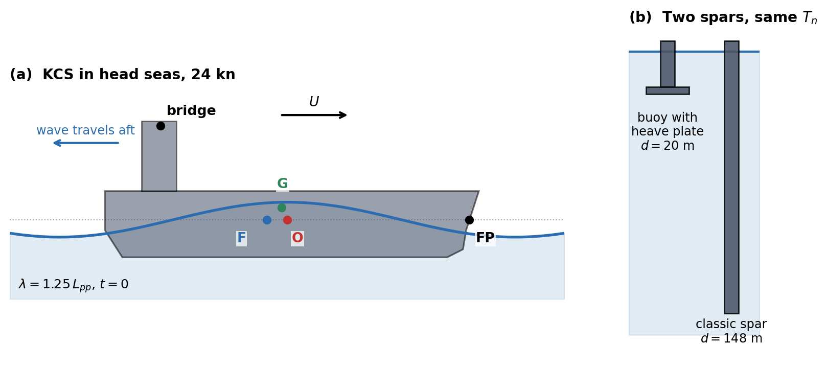
Figure 8.1 shows the KCS in the wave of Problems 1 and 3, and the two spars to scale.
Reading an RAO. The KCS steams at \(24\) kn in head seas (\(\beta = 180^{\circ}\)) in a regular wave of length \(\lambda = 1.25\,L_{pp}\). At this wave the motion RAOs at \(O\) are \[\frac{\hat\xi_3}{A} = 1.151 - 0.691i, \qquad \frac{\hat\xi_5}{kA} = -0.932 - 0.330i.\]
- Find \(\omega\), \(\omega_e\) and the encounter period \(T_e\). Write each RAO as a magnitude and a phase, and state the units of \(\hat\xi_3/A\), \(\hat\xi_5/A\) and \(\hat\xi_5/(kA)\). Express the pitch RAO in degrees per metre of wave amplitude, and give the heave and pitch amplitudes in a wave of height \(H = 6\) m. The KCS was tested in the towing tank as a \(1:31.6\) scale model. Explain why the RAO \(\hat\xi_5/(kA)\) measured on the model applies unchanged to the ship, while the same RAO in degrees per metre does not.
- At \(t = 0\) the crest is at \(O\). Find the times, within one encounter period, at which the heave reaches its highest point and the pitch its largest bow-down angle, and say whether each leads or lags the crest. A phase of \(-160^{\circ}\) is the same as one of \(+200^{\circ}\): is the pitch then lagging the crest by \(160^{\circ}\) or leading it by \(200^{\circ}\)? Finally, describe the ship at \(t = 0\): is \(O\) above or below its mean position, and moving up or down? Is the bow up or down, and turning which way? Explain this attitude from where the crest was a few seconds earlier.
- In very long waves the ship follows the water surface. From that picture alone, show that in head seas \(\hat\xi_3/A \rightarrow 1\) with zero phase and \(\hat\xi_5/(kA) \rightarrow 1\) with a phase of \(-90^{\circ}\), in the conventions of this book. A colleague’s seakeeping code reports a long-wave pitch phase of \(+90^{\circ}\) in head seas. Name two independent differences of convention, each of which would produce this. Show that a code with both differences reports \(-90^{\circ}\) and passes the check. Design a check, using the heave phase from (a), that tells the two apart. Name a third difference that no long-wave check can ever detect.
- In the towing tank the incident wave is measured by a probe fixed to the carriage, a distance \(x_p\) ahead of \(O\); take \(x_p = 100\) m at full scale. Show that the RAO relative to the probe signal is the RAO at \(O\) multiplied by \(e^{ikx_p\cos\beta}\). Evaluate the change of phase for the wave of (a), and give the heave and pitch phases relative to the probe. A student argues instead that the crest takes \(x_p/(c + U)\) to travel from the probe to \(O\), where \(c\) is the phase speed, and multiplies this delay by \(\omega_e\). Show that the two arguments agree. Why does the shift depend on \(k\) and not on \(\omega_e\), even though the ship meets the waves at \(\omega_e\)?
- The heave RAO in (a) is greater than one. A student objects that a ship cannot rise higher than the water it floats in. Find how far \(O\) stands above the local water surface at the moment of greatest heave, and the amplitude of the relative motion between \(O\) and the water surface. Explain what the student has confused. Is the long wave limit of (c) a bound?
Heave of the KCS in head seas: the uncoupled estimate, the reference point, and forward speed. The tables below are from the HydRA run, in head seas. The loads are per unit \(\rho gAA_{WP}\), which is \(C_{33}A\), so they are dimensionless. \(\zeta_{33} = B_{33}/\left(2\sqrt{C_{33}(m + A_{33})}\right)\), and the RAOs are those of the full coupled \(6\times6\) solution. The uncoupled zero speed heave natural frequency is \(\omega_n = 0.743\) rad/s.
Table A — zero speed:
\(\omega\) (rad/s) \(\hat F_3/(C_{33}A)\) \(A_{33}/m\) \(\zeta_{33}\) \(\hat\xi_3/A\) \(\hat\xi_5/A\) (\(10^{-3}\) rad/m) 0.39 \(0.4157 + 0.0608i\) 2.014 0.177 \(0.6705 + 0.0417i\) \(-2.611 - 12.60i\) 0.48 \(0.1685 + 0.0593i\) 1.485 0.209 \(0.3643 + 0.1382i\) \(-4.749 - 13.43i\) 0.51 \(0.0909 + 0.0537i\) 1.370 0.210 \(0.2584 + 0.1750i\) \(-5.053 - 12.40i\) 0.60 \(-0.0726 + 0.0206i\) 1.199 0.197 \(-0.0416 + 0.2547i\) \(-2.425 - 6.743i\) 0.75 \(-0.0536 - 0.0346i\) 1.105 0.174 \(-0.1844 + 0.2093i\) \(5.496 - 1.001i\) Table B — \(24\) kn, with \(A_{33}\) and \(\zeta_{33}\) at the encounter frequency:
\(\omega\) (rad/s) \(\omega_e\) (rad/s) \(\hat F_3/(C_{33}A)\) \(A_{33}/m\) \(\zeta_{33}\) \(\hat\xi_3/A\) \(\hat\xi_5/A\) (\(10^{-3}\) rad/m) 0.39 0.5815 \(0.4444 + 0.0578i\) 1.219 0.200 \(1.144 - 0.019i\) \(-10.97 - 13.20i\) 0.48 0.7701 \(0.1550 + 0.0126i\) 1.096 0.170 \(0.834 - 0.926i\) \(-21.08 - 2.254i\) 0.51 0.8375 \(0.0609 + 0.0014i\) 1.081 0.154 \(0.130 - 0.755i\) \(-15.84 + 5.489i\) Table C — heave–pitch coefficients at \(\omega_e = 0.7701\) rad/s (in units of \(10^{6}\): kg, N·s/m, kg·m, N·s):
\(A_{33}\) \(B_{33}\) \(A_{35}\) \(A_{53}\) \(B_{35}\) \(B_{53}\) \(U = 0\) 58.10 28.18 1003 1007 527.0 522.4 \(24\) kn, head seas, \(\omega = 0.48\) 58.10 28.18 416.6 1594 1244 \(-194.9\) - Treat heave as a single degree of freedom. Show that its RAO factorises as \(\hat F_3/(C_{33}A)\), which depends only on the hull and the wave, times a dynamic amplification factor which depends only on the ship’s mass, added mass, damping and stiffness. Evaluate both factors and the uncoupled RAO at the five frequencies of Table A. The heave natural frequency lies inside the range of the table, yet the zero speed heave RAO has no resonant peak and never exceeds one. Explain why, using the two factors and the wavelength at \(\omega_n\).
- Compare your uncoupled RAO with the coupled \(\hat\xi_3/A\). Now compute the heave of the centre of flotation \(F\), \(\hat\xi_3 - x_F\hat\xi_5\). Show from the hydrostatics that \(x_F = -C_{35}/C_{33}\), and evaluate it. Compare the heave of \(F\) with your uncoupled estimate, and explain the result. What is the “coupling” in the coupled heave at \(O\) mostly made of? Why is the agreement not exact? Use the zero speed values of Table C and the position of \(G\) to locate the centroids of the added mass and of the mass plus added mass.
- Repeat the uncoupled estimate and the heave of \(F\) at \(24\) kn, using Table B and \(\omega_e\) throughout. Both now fail badly. By how much, and at which frequency?
- Write the heave row of the coupled equations at \(\omega = 0.48\) rad/s, keeping only heave and pitch, with \(M_{35} = -mx_G\) from Chapter 5. Using Tables B and C, evaluate the terms \(Z_{33}\hat\xi_3\) and \(Z_{35}\hat\xi_5\) and check that their sum is close to \(\hat F_3\). Compare \(|Z_{35}\hat\xi_5|\) with \(|\hat F_3|\). From Table C, show that forward speed has changed the coefficients by \(A_{35} - A_{35}^{(0)} = -(U/\omega_e^2)B_{33}\), \(B_{35} - B_{35}^{(0)} = +UA_{33}\), and by the opposite amounts for \(A_{53}\) and \(B_{53}\). Hence show that the speed-dependent part of \(Z_{35}\) is \(U\left(B_{33} + i\omega_eA_{33}\right)\), and interpret this term as the heave force on a hull that is pitched and moving forward, using the vertical velocity that a pitched hull moving at \(U\) imposes on the water beneath it. How large is the heave force it produces here, compared with the wave force?
- At zero speed \(A_{35} \approx A_{53}\), at \(24\) kn they differ by a factor of four. Which property of the zero speed radiation problem makes the matrices symmetric, and what replaces it at forward speed? A student “cleans up” the forward speed matrices by replacing each off-diagonal pair by its average, on the grounds that physical matrices must be symmetric. Which part of the physics in (d) has the student removed?
Where the motion is felt: green water, slamming and the wheelhouse. The KCS is in the wave of Problem 1 (\(\lambda = 1.25\,L_{pp}\), head seas). At \(24\) kn the RAOs are as given there. At \(12\) kn (\(U = 6.17\) m/s) in the same wave they are \(\hat\xi_3/A = 0.751 + 0.093i\) and \(\hat\xi_5/(kA) = -0.562 - 0.630i\). The forward perpendicular (FP) is at \(x = 115\) m. Take the draft there as \(10.8\) m and the freeboard to the deck as \(D - T = 8.2\) m, ignoring sheer and flare. Assume the wheelhouse is at \(x = -80\) m.
- Show that to first order the vertical displacement of a point \(P = (x, y, z)\) of the hull is \(\xi_3 + y\xi_4 - x\xi_5\). Evaluate the vertical motion RAO at the FP at \(24\) kn, and compare its magnitude with \(|\hat\xi_3/A| + 115\,|\hat\xi_5/A|\). Which is right, and why are they different? Find the point \(x^*\) along the centreline where the vertical motion is smallest, and its RAO there.
- The relative motion \(r = s_3 - \eta\), between the hull and the local water surface, decides whether the deck is wetted or the forefoot leaves the water. Here \(s_3\) is the vertical displacement of the hull. Evaluate the relative motion RAO at the FP, ignoring the disturbance of the water surface by the ship. Find the wave amplitude at which green water first comes over the bow, and the amplitude at which the forefoot first emerges. Which happens first? Emergence alone does not make a slam: the keel must also re-enter faster than a threshold, commonly taken as \(0.093\sqrt{gL}\) (Ochi’s criterion). In a regular wave with relative motion amplitude \(r_a\), show that the re-entry velocity is \(\omega_e\sqrt{r_a^2 - T^2}\). Hence find the wave amplitude at which the bow begins to slam.
- The master reduces speed to \(12\) kn. Repeat (b) at \(12\) kn. Compare also the vertical acceleration at the FP per metre of wave amplitude at the two speeds, as a fraction of \(g\). Explain the improvement in terms of \(\omega_e\) and of the phases. Why is the gain larger than the change of the heave RAO alone suggests?
- Seakeeping criteria limit the RMS vertical acceleration in the wheelhouse to about \(0.15g\). In a regular wave the RMS value is the amplitude divided by \(\sqrt2\). Find the wave amplitude at which this limit is reached at \(24\) kn and at \(12\) kn. Where along the ship would you put the accommodation, and why?
- If (b) predicts that the forefoot emerges, at least one assumption of the linear theory used to compute it has failed. Which? Name the loads on the hull that appear as a result, which the RAO cannot describe. Explain also why the true relative motion at the bow is usually larger than your estimate, even when the bow stays in the water.
The modes with no spring: surge, sway and yaw.
- In long waves the horizontal exciting force on a hull is its displaced mass plus its added mass, times the horizontal acceleration of the undisturbed water (Problems 5 and 9 of Chapter 7). Using this, show that at forward speed the long wave surge RAO tends to \((\omega/\omega_e)^2|\cos\beta|\), not to \(|\cos\beta|\). Explain why the wave frequency sets the load while the encounter frequency sets the response. For the KCS at \(24\) kn with \(\lambda = 2L_{pp}\), evaluate the factor \((\omega/\omega_e)^2\) in head and in following seas. The explorer gives \(|\hat\xi_1/A| = 0.781\) (head) and \(0.782\) (following) at zero speed, and \(0.417\) (head) and \(2.360\) (following) at \(24\) kn. Compare the ratios with your factor and explain the difference.
- In following seas \(\omega_e \rightarrow 0\) at \(\omega = g/U\). For the KCS at \(24\) kn, find this wave’s frequency, length and phase speed, and say what the linear surge RAO predicts there. Describe what really happens to a ship that a steep wave overtakes this slowly (surf-riding). Which forces decide the outcome, and why are they absent from the equations of this chapter? Show that the wave whose phase speed equals the ship speed has \(\lambda/L = 2\pi Fn^2\). IMO’s second generation intact stability criteria regard a ship as potentially vulnerable to surf-riding only if \(L < 200\) m and \(Fn > 0.3\). Find the Froude number of the KCS at \(24\) kn, and use your result to explain why the screening rests on \(Fn\) and singles out short, fast ships.
- Sway and yaw have no restoring force either. An autopilot that applies rudder in proportion to the heading error and its rate adds a yaw moment \(N = -K_p\xi_6 - K_d\dot\xi_6\). Show where \(K_p\) and \(K_d\) enter the frequency domain equations, and that yaw acquires a natural frequency. Why does the yaw RAO now stay finite as \(\omega_e \rightarrow 0\)? Why can a real ship in steep quartering seas still broach, swinging broadside to the waves against full rudder? Which mode is still free?
- A turret-moored FPSO has \(m = 3.0\times10^{8}\) kg, a surge added mass of \(5\%\) of \(m\), and a mooring surge stiffness \(K_{11} = 5.5\times10^{5}\) N/m. Find its surge natural period, and the length of a regular wave with that period. Compare \(K_{11}\) with \(\omega^2(m + A_{11})\) for a \(10\) s wave, and explain why the moorings play no part in the wave frequency motions. Yet the mooring lines are designed for large surge excursions at the natural period. A sea contains two components of periods \(10.0\) s and \(10.7\) s. Show that the square of the elevation, which drives the second order drift force of Problem 1(d) of Chapter 7, contains a term at the difference frequency, and find its period. Explain how a sea with no energy at \(150\) s can drive a \(150\) s resonance, and why this resonance is so lightly damped.
Roll: the damping the panel method cannot see. Use the KCS data given at the start of these exercises.
- Find the roll natural frequency and period, \(GM_T\), the critical roll damping \(B_{cr} = 2\sqrt{C_{44}(I_{44} + A_{44})}\) and the wave-making damping ratio. With wave-making damping alone, by what factor does resonance amplify the static roll? Why is the wave-making roll damping of a ship-shaped hull so small, when its heave damping (Problem 2) is near \(20\%\) of critical?
- At \(24\) kn in stern quartering seas (\(\beta = 45^{\circ}\)), the ship meets two different wave frequencies at the encounter frequency \(\omega_e = \omega_n\) of roll. Find both, with their periods and lengths, and say which lies in the \(5\)–\(20\) s band that carries most of the energy of a wind sea. At the shorter wave, HydRA gives a roll exciting moment of \(|\hat F_4|/A = 24.6\) MN·m per metre. Estimate the resonant roll RAO with \(\zeta = 0.05\) as a single degree of freedom, in degrees per metre and per unit wave slope. The coupled explorer gives \(41.9^{\circ}\)/m. Comment on the difference, and on the size of the result for a wave of \(1\) m amplitude and \(72\) m length.
- Roll damping is not linear. Decay tests show an equivalent damping ratio of \(0.05\) at \(10^{\circ}\) amplitude, with the damping moment quadratic in the roll velocity, \(B_q|\dot\xi_4|\dot\xi_4\). By equating the energy dissipated per cycle, show that the equivalent linear damping is \(B_{eq} = \frac{8}{3\pi}\omega\xi_aB_q\), so that the equivalent damping ratio is proportional to the roll amplitude \(\xi_a\). Find the resonant roll amplitude in the wave of (b) for \(A = 0.5\), \(1\) and \(2\) m, and show that it grows as \(\sqrt{A}\). What becomes of the RAO? A roll RAO measured with \(A = 0.5\) m is used to predict roll at \(A = 2\) m: by what factor, and in which direction, is the prediction wrong?
- A container sits at the top of a deck stack, \(30\) m above the waterline on the centreline. The ship rolls about \(O\) with amplitude \(\xi_a = 22^{\circ}\) at the encounter period of (b). Show that at the extreme of roll the lateral force per unit mass on the container, in the ship’s axes, is to first order \((g + z\omega_e^2)\xi_a\), with gravity and inertia acting towards the low side. Evaluate both parts. Repeat for a stiffer loading condition with a roll period of \(20\) s. What does this say about where the danger to deck cargo lies? Why does a lateral accelerometer on the bridge register \(g\xi_4\) even in very slow roll?
- Name the physical sources of roll damping that a potential flow panel method omits, and say for each why potential flow cannot produce it. Which grows with forward speed, and why? Why do bilge keels, small as they are, change the roll RAO more than almost any other feature of the hull?
Parametric roll: an RAO of zero, and forty degrees of roll. In October 1998 the post-Panamax container ship APL China met a storm in the North Pacific while heading into the waves at reduced speed. She rolled to angles reported at up to \(35\)–\(40^{\circ}\), and lost or damaged a large part of her deck cargo. The investigations that followed identified parametric roll in head seas as the cause.
- Show that linear theory predicts no roll at all for a ship symmetric about its centreplane in head seas. Use the symmetry of the wave loads (Problem 1(e) of Chapter 7) and the structure of \(\boldsymbol{M}_{RB}\), \(\boldsymbol{A}\), \(\boldsymbol{B}\) and \(\boldsymbol{C}\) (Chapter 6). Is it right to say that “the linear roll RAO is inaccurate in head seas”?
- With a crest of a wave of length \(\lambda = L\) amidships, the bow and the stern sit in troughs, and half an encounter period later the reverse. Show that for a wall-sided hull the transverse moment of inertia \(I_T\) of the waterplane does not change. A container ship has strong flare at the bow and a wide, flat stern. Model each end quarter of the KCS waterplane by a mean half-breadth \(b = 10\) m with sides flared outwards at \(\theta = 30^{\circ}\) from the vertical, and take the middle half as wall-sided. Estimate the change of \(GM_T\) with a crest of amplitude \(A_w = 4\) m amidships. Ignore the heave and pitch of the hull relative to the wave.
- With \(GM_T\) varying as \(GM_T(1 + \epsilon\cos\omega_et)\), write the roll equation of motion. It is a Mathieu equation. Show that roll at a frequency \(\omega_e/2\) makes the varying restoring moment produce a moment at \(\omega_e/2\) itself, so the motion can feed itself, most effectively when \(T_e = T_R/2\). Balance the work done over one roll cycle by the varying restoring moment against the energy dissipated by damping, and show that roll grows only if \(\epsilon > 4\zeta\). At which step of the linearisation in this chapter was this term discarded, and why can no linear time-invariant system produce a response at half the forcing frequency?
- The loading condition of this chapter has \(GM_T = 0.55\) m and \(T_R = 38.9\) s. A heavier loading condition of the same ship has \(GM_T = 2.0\) m and the same roll inertia. Find its \(T_R\). For each condition, find the speed at which \(T_e = T_R/2\) is met in waves with \(\lambda = L_{pp}\), in head seas and in following seas. Check the threshold of (c) with \(\zeta = 0.05\) and the \(\epsilon\) from (b). Which condition is at risk, at what speed and heading? Why might a master choose exactly that speed deliberately (Problem 3)?
- For the \(GM_T = 0.55\) m condition, (b) predicts something more alarming than a varying \(GM_T\) when the crest is amidships. What is it, and in which conditions of speed and heading would it last long enough to matter (Problem 4(b))? Name two practical countermeasures against parametric roll, one operational and one in the design.
Two ways to keep a spar still. Take the spar buoy with its heave plate and the classic spar described at the start of these exercises, both with \(\zeta = 0.05\).
- Write the heave RAO of the buoy, and show that it tends to one in long waves. Find its heave natural period \(T_n\) and the period \(T^*\) at which its heave exciting force vanishes (Problem 7(d) of Chapter 7). Evaluate the magnitude of the RAO at \(T = 8\), \(12\), \(16\) and \(20\) s, at \(T^*\), at \(T_n\) and at \(30\) s. Find its largest value and the period at which it occurs. Explain why the largest response is not at \(T_n\).
- Find the draft of the classic spar that gives it the same \(T_n\), and write its heave RAO. Show that at its natural frequency the exciting force is \(e^{-1}\) of its long wave value, whatever the draft, so that its resonant RAO is close to \(1/(2\zeta e)\). Compare the two spars at resonance, and at \(T = 12\) s, typical of the peak period of a storm sea. What does the classic spar’s draft buy, and what can no amount of draft buy?
- Find the largest heave RAO of each spar for \(\zeta = 0.02\), \(0.05\) and \(0.10\). Which design is more sensitive to the damping, and why? Why does that matter, given that \(\zeta\) is the least certain number in the whole calculation?
- The added mass of the plate is an estimate. Recompute \(T_n\), \(T^*\) and the largest RAO of the buoy if \(A_{33}\) is \(20\%\) larger, and \(20\%\) smaller. Does the design still work? Explain why \(T_n\) and \(T^*\) move in the same direction, and why that makes the design robust.
- A designer of a wave energy converter wants the opposite: a large heave motion at \(T = 8\) s, the peak period of the local sea. For a plain floating cylinder, find the draft that tunes it to \(8\) s, and show that its resonant RAO is again about \(1/(2\zeta e)\), whatever its diameter. Split the damping into a power take-off part \(B_{PTO}\) and the rest, \(B_0\), which includes radiation. Show that the power absorbed at resonance, \(P = \tfrac12B_{PTO}\omega^2|\hat\xi_3|^2\), is greatest when \(B_{PTO} = B_0\). Explain why the heave plate of the buoy is exactly what this designer must avoid.
Impulse responses: why the motion starts before the wave.
- For a plain vertical column of draft \(d\) in long waves, the heave exciting force per unit amplitude is \(\rho gA_ce^{-kd}\) with \(k = \omega^2/g\). Show that the impulse response from the wave elevation at the axis to the heave force is a Gaussian, \(f(t) = \rho gA_c\,e^{-t^2/(4a)}/\sqrt{4\pi a}\) with \(a = d/g\). Show that it is even in time, find its area, and give its width \(\sigma = \sqrt{2a}\) for the classic spar and for a hull of the KCS draft.
- The force begins well before the impulse in the elevation at \(O\) arrives. Explain why this does not violate causality, using the dispersion of deep water waves. What must the sea have looked like before \(t = 0\) if the elevation at \(O\) is to be a delta function at \(t = 0\)?
- The heave impulse response of the classic spar is the convolution of \(f(t)\) with the causal impulse response of Chapter 3, from force to heave. Show that it is non-zero before \(t = 0\), but negligible before about \(t = -3\sigma\). Compute the fraction of \(\int h^2\,dt\) at negative times. Explain, using \(T_n\), why the spar’s heave impulse response is nearly causal, while that of the KCS in head seas at zero speed has about \(60\%\) of its energy at negative times (see the impulse response explorer). For the KCS, estimate the time a crest takes to travel from the FP to \(O\) at zero speed, for a wave at the heave natural frequency, and compare it with \(\sigma\) for the KCS draft. Which dominates the non-causality of a ship’s impulse response, its draft or its length?
- Crane operations offshore and helicopter landings on ships rely on predicting the motion a few seconds ahead. Explain why a perfect measurement of the elevation at \(O\), up to the present, cannot predict the motion even at the present instant. A wave radar measures the sea a distance \(D\) up-wave of the classic spar. Using the group velocity \(c_g = g/(2\omega)\), show that the prediction horizon is set by the longest waves that matter. If waves with \(\omega \geq 0.3\) rad/s matter, how large must \(D\) be to predict the heave \(10\) s ahead, allowing for the precursor of (c)?
- In long waves the surge RAO tends to \(-i|\cos\beta|\) in following seas (see the impulse response explorer). Using \(\hat h(-\omega) = \hat h^*(\omega)\), show that an RAO equal to \(-iH_0\) at all positive frequencies has the impulse response \(H_0/(\pi t)\), which decays only as \(1/t\) on both sides of \(t = 0\). Why is this unavoidable for a body with no surge restoring force? Propose a way of computing surge time histories that avoids such a slowly decaying kernel.
Programming Problem: From RAO to time history. Write the code for this problem yourself; the RAOs of the two spars are given in closed form at the start of these exercises.
- Write a function that evaluates \(h(t) = \frac{1}{\pi}\int_0^{\infty}\operatorname{Re}\left(\hat h(\omega)e^{i\omega t}\right)d\omega\) by the trapezoidal rule. Apply it to the heave RAOs of both spars, with \(\Delta\omega = 0.0005\) rad/s up to \(2\) rad/s, for \(-150 \leq t \leq 450\) s. For the classic spar, check the result against an independent calculation: the numerical convolution of the Gaussian of Problem 8(a) with the causal force-to-heave impulse response. For both, check that \(\int h\,dt = \hat h(0)\), and find the fraction of \(\int h^2\,dt\) at negative times.
- A focused wave group arrives at \(O\): \(\eta(t) = \sum_na_n\cos\omega_nt\), with \(a_n \propto \exp\left[-(\omega_n - \omega_p)^2/(2s^2)\right]\), \(\omega_p = 2\pi/12\) rad/s and \(s = 0.08\) rad/s, scaled so that the crest at \(O\) at \(t = 0\) is \(10\) m high. Compute the heave of both spars in two ways: (i) by superposing the RAO responses to each component, and (ii) by convolving \(\eta(t)\) with \(h(t)\). Show that they agree. Give the largest heave of each spar and the time at which it occurs. Then repeat (ii) with \(h(t)\) set to zero for \(t < 0\). How large is the error made by forcing causality on each spar?
- Repeat (a) for the buoy with \(\zeta = 0.01\), but with a coarse step \(\Delta\omega = 0.05\) rad/s. Values appear well before \(t = 0\) that were not there before. Explain where they come from, and how to tell this artefact from the genuine non-causality of (a) without knowing the answer in advance.
- Cut the buoy’s RAO (\(\zeta = 0.05\)) off abruptly at \(\omega_c = 0.8\) rad/s and recompute \(h(t)\). Describe the error, and relate its period to \(\omega_c\). Then apply a cosine taper that takes the RAO smoothly to zero between \(0.6\) and \(0.8\) rad/s. Does the taper cure the problem? Which features of the truncated \(h(t)\) are physical, which are produced by the cut-off, and what is the real cure?
- Both spars have the same \(T_n\) and the same \(\zeta\), so their impulse responses decay at the same rate. Compare the amplitudes of their ringing after the first \(100\) s, and explain the ratio from the RAOs alone, without the time domain calculation.
Answer Key
Problem 1 — Reading an RAO
(a) An RAO is a complex number: its magnitude is the motion per unit of wave, its phase is the timing of the motion relative to the crest at \(O\).
Wave and encounter. \(\lambda = 287.5\) m, \(k = 2\pi/\lambda = 0.02185\) m\(^{-1}\), \(\omega = \sqrt{gk} = 0.4630\) rad/s. In head seas the ship runs into the waves:\[\omega_e = \omega + \frac{\omega^2}{g}U = \omega + kU = 0.7329\ \text{rad/s},\]so \(T_e = 8.57\) s, against a wave period of \(13.57\) s.
Magnitude and phase.\[\frac{\hat\xi_3}{A} = 1.342\angle-31.0^\circ\]\[\frac{\hat\xi_5}{kA} = 0.989\angle-160.5^\circ\]
Units. \(kA\) is the largest slope of the water surface, so dividing a rotation by it gives a pure number:\[\begin{array}{l|l} \text{RAO} & \text{units} \\ \hline \hat\xi_3/A & \text{m/m (dimensionless)} \\ \hat\xi_5/A & \text{rad/m} \\ \hat\xi_5/(kA) & \text{rad/rad (dimensionless)} \end{array}\]
Per metre of wave. \(|\hat\xi_5/A| = k\times0.989 = 0.02161\) rad/m \(= 1.238^\circ\)/m. In a wave of height \(H = 6\) m (\(A = 3\) m): heave \(4.03\) m, pitch \(3.71^\circ\).
Model and ship. Froude scaling with \(s = 31.6\) divides every length by \(s\) and leaves angles unchanged. \(A\) becomes \(A/s\) and \(k\) becomes \(sk\), so the slope \(kA\) and the pitch angle are both unchanged: \(\hat\xi_5/(kA)\) is the same number for model and ship. In degrees per metre the model’s RAO is \(31.6\) times the ship’s, because a metre of wave is \(31.6\) times larger relative to the model.
Takeaway. Rotations are quoted per unit wave slope because that form does not depend on scale.
(b) Read a phase as a delay: a phase of \(-\varphi\) puts the maximum \(\varphi/360^\circ\) of an encounter period after the crest passes \(O\).
Highest heave. \(\xi_3(t) = 1.342A\cos(\omega_et -31.0^\circ)\) peaks when \(\omega_et = 31.0^\circ\), at \(t = 0.74\) s: heave lags the crest by \(31^\circ\).
Largest bow-down pitch. At \(\omega_et = 160.5^\circ\), \(t = 3.82\) s. The largest bow-up angle comes half a cycle earlier, \(19.5^\circ\) or \(0.46\) s before the crest reaches \(O\).
Lag or lead? Phases are defined only modulo \(360^\circ\), so a lag of \(160^\circ\) and a lead of \(200^\circ\) are the same statement. Lead and lag are a convention, by which the phase is quoted in \((-180^\circ, 180^\circ]\); they say nothing about cause and effect.
The ship at \(t = 0\). Take real parts of \(\hat\xi e^{i\omega_et}\) and of its time derivative \(i\omega_e\hat\xi e^{i\omega_et}\):\[\begin{array}{l|l|l} \text{quantity at } t = 0 & \text{value} & \text{meaning} \\ \hline \xi_3 = \operatorname{Re}\hat\xi_3 & +1.151\,A & O\ \text{above its mean} \\ \dot\xi_3 = \operatorname{Re}(i\omega_e\hat\xi_3) & +0.691\,\omega_eA & \text{still rising} \\ \xi_5 = \operatorname{Re}\hat\xi_5 & -0.932\,kA & \text{bow up} \\ \dot\xi_5 = \operatorname{Re}(i\omega_e\hat\xi_5) & +0.330\,\omega_ekA & \text{turning bow-down} \end{array}\]
Why. The crest moves aft relative to the ship at \(c + U = 21.19 + 12.35 = 33.54\) m/s, so it passed the FP \(3.43\) s earlier. It lifted the bow; now that it is amidships, the bow has just passed its highest point and is starting to fall, while the hull as a whole is still being lifted (figures below).


(c) In long waves the hull is a raft on the surface. That picture alone fixes both long-wave limits, and gives a test of any code’s conventions.
Following the surface. Every point of the waterline rises with the local elevation: \(\xi_3 - x\xi_5 = \eta(x)\) along the whole hull. In head seas \(\hat\eta = Ae^{-ikx\cos\beta} = Ae^{ikx}\).
Heave. At \(x = 0\): \(\hat\xi_3 = A\), magnitude one, phase zero.
Pitch. Differentiate in \(x\) at \(x = 0\):\[-\hat\xi_5 = \frac{\partial\hat\eta}{\partial x} = ikA\]\[\hat\xi_5 = -ikA,\]magnitude \(kA\), phase \(-90^\circ\). Physically: a quarter period after the crest passes \(O\), the downslope towards the bow lies under \(O\), so the bow is down.
Two conventions that each give \(+90^\circ\). (i) A time factor \(e^{-i\omega t}\), which reverses the sign of every phase. (ii) Pitch positive bow up, which adds \(180^\circ\) to the pitch phase only. A code with both reports \(-(-90^\circ) + 180^\circ \equiv -90^\circ\) and passes the long-wave check while disagreeing with this book twice.
Telling them apart. Use the heave phase of (a), \(-31^\circ\):\[\begin{array}{l|c|c} \text{code} & \text{heave phase in (a)} & \text{long-wave pitch} \\ \hline \text{this book} & -31^\circ & -90^\circ \\ \text{(i) only} & +31^\circ & +90^\circ \\ \text{(ii) only} & -31^\circ & +90^\circ \\ \text{(i) and (ii)} & +31^\circ & -90^\circ \end{array}\]Convention (ii) does not touch heave, so the sign of the heave phase identifies (i).
The invisible third. The phase reference point. A code that puts the crest at the FP or at \(G\) at \(t = 0\) multiplies every RAO by \(e^{ikx_{\text{ref}}\cos\beta}\), which tends to one as \(k \rightarrow 0\). Two codes can agree perfectly in long waves and differ by tens of degrees at \(\lambda \approx L\). The check of Problem 10(d) of Chapter 7 applies to motions too.
(d) Moving the phase reference from \(O\) to the probe shifts every phase by the number of wavelengths between them; the magnitudes do not change.
The shift. In the frame moving with the ship, \(\hat\eta(x, y) = Ae^{-ik(x\cos\beta + y\sin\beta)}\) with time factor \(e^{i\omega_et}\). The probe measures \(\hat\eta_p = Ae^{-ikx_p\cos\beta}\), so\[\frac{\hat\xi}{\hat\eta_p} = \frac{\hat\xi}{A}\,e^{ikx_p\cos\beta}.\]
Values. In head seas \(kx_p\cos\beta = -125.2^\circ\). Relative to the probe, heave is at \(-156.2^\circ\) and pitch at \(74.3^\circ\). The probe is ahead and sees each crest first, so the motion lags the probe by more than it lags the crest at \(O\).
The student’s argument. Delay \(x_p/(c + U) = 2.982\) s, and \(\omega_e\,x_p/(c + U) = 125.2^\circ\), the same number. Algebraically, \(\omega_e = \omega + kU = k(c + U)\), so\[\frac{\omega_ex_p}{c + U} = kx_p\quad\text{exactly.}\]
Why \(k\), not \(\omega_e\). The shift is a spatial phase. In the moving frame the wave pattern keeps its shape, with crests \(\lambda\) apart, and only its rate of passage depends on \(U\). The phase difference between two points fixed to the ship is the number of wavelengths between them.
(e) An RAO above one is the overshoot of a spring–mass system, not the hull leaving the water that supports it.
At greatest heave (\(t = 0.74\) s). The water at \(O\) stands at \(A\cos(\omega_et) = 0.857A\) and \(O\) at \(1.342A\): \(O\) is \(0.485A\) above the local surface (figure above, right).
Relative motion at \(O\). \(|\hat\xi_3/A - 1| = 0.707\) per metre. The hull rises out of the wave and sinks back in, and that change of immersion is exactly what the hydrostatic and hydrodynamic forces respond to.
The confusion. The student has taken the quasi-static limit of (c) for an upper bound. In long waves the ship has time to settle on the local surface and the RAO tends to one. Near resonance it is a mass on a spring driven close to its natural frequency, here \(\omega_e = 0.733\) rad/s against a heave natural frequency of \(0.743\) rad/s, and a spring–mass system overshoots its static deflection (Chapter 2). At \(24\) kn there is a second reason, the coupling with pitch: Problem 2.
Problem 2 — Heave of the KCS in head seas
(a) The heave RAO is (how hard the wave pushes) times (how much the ship amplifies a push). At zero speed the two are never large at the same frequency.
Factorisation. With one degree of freedom, \(\left[C_{33} - \omega^2(m + A_{33}) + i\omega B_{33}\right]\hat\xi_3 = \hat F_3\). Divide by \(C_{33}A\):\[\frac{\hat\xi_3}{A} = \underbrace{\frac{\hat F_3}{C_{33}A}}_{\text{load}}\;\underbrace{\frac{1}{1 - \omega^2\dfrac{m + A_{33}}{C_{33}} + 2i\zeta_{33}\,\omega\sqrt{\dfrac{m + A_{33}}{C_{33}}}}}_{\text{dynamic amplification}}\]The load is the heave force the hull extracts from the wave, relative to the static force of a long wave: geometry and wavelength only. The second factor is the DAF of Chapter 2, with frequency-dependent coefficients.
Values.\[\begin{array}{c|c|c|c|c} \omega & |\text{load}| & |\text{DAF}| & \hat\xi_3/A\ \text{(uncoupled)} & |\hat\xi_3/A| \\ \hline 0.39 & 0.420 & 1.549 & 0.637 - 0.133i & 0.651 \\ 0.48 & 0.179 & 1.704 & 0.299 - 0.0559i & 0.304 \\ 0.51 & 0.106 & 1.782 & 0.188 - 0.00798i & 0.188 \\ 0.60 & 0.075 & 2.193 & -0.0795 + 0.145i & 0.165 \\ 0.75 & 0.064 & 2.846 & -0.091 + 0.157i & 0.182\end{array}\]
Why no peak. Resonance at \(\omega_n = 0.743\) rad/s is met in waves of length \(2\pi g/\omega_n^2 = 112\) m \(= 0.49\,L_{pp}\). The crests and troughs along a ship twice that long nearly cancel, as for the barge at \(\lambda = L/2\) in Chapter 7, so the load is only \(0.064\). The amplification there is about \(1/(2\zeta_{33}) = 2.9\), modest because heave radiates waves efficiently. The product is \(0.18\). In long waves the load tends to one, but so does the amplification (figure below, left).
Takeaway. At zero speed, the wave that could excite heave resonance is too short to push the ship, and the wave that pushes it hardest is too long to excite resonance.
(b) Most of the coupling in the heave at \(O\) is geometry: measured at the centre of flotation, heave is nearly uncoupled.
Where \(F\) is. A strip of waterplane at \(x\) rises by \(\xi_3 - x\xi_5\), so the hydrostatic heave force is\[-\rho g\iint(\xi_3 - x\xi_5)\,dA = -\rho gA_{WP}\,\xi_3 + \rho g\left(\iint x\,dA\right)\xi_5.\]Hence \(C_{33} = \rho gA_{WP}\) and \(C_{35} = -\rho gA_{WP}x_F\), so \(x_F = -C_{35}/C_{33} = -12.77\) m: \(F\) is \(12.8\) m aft of midship.
Heave at \(O\) and at \(F\).\[{\small\begin{array}{c|c|c|c} \omega & \text{uncoupled} & \hat\xi_3/A\ \text{at } O & \text{heave of } F \\ \hline 0.39 & 0.637 - 0.133i & 0.67 + 0.0417i & 0.637 - 0.119i \\ 0.48 & 0.299 - 0.0559i & 0.364 + 0.138i & 0.304 - 0.0333i \\ 0.51 & 0.188 - 0.00798i & 0.258 + 0.175i & 0.194 + 0.0166i \\ 0.60 & -0.0795 + 0.145i & -0.0416 + 0.255i & -0.0726 + 0.169i \\ 0.75 & -0.091 + 0.157i & -0.184 + 0.209i & -0.114 + 0.197i\end{array}}\]with the heave of \(F\) computed as \((\hat\xi_3 - x_F\hat\xi_5)/A\).
Reading. The uncoupled estimate is up to \(40\%\) below the heave at \(O\) near \(\lambda \approx L\), but it reproduces the heave of \(F\) to within a few percent for \(\lambda \gtrsim L\), and much more closely than at \(O\) in the shorter waves. The coupling is mostly kinematic: the ship pitches roughly about \(F\), and a point \(12.8\) m forward of \(F\) moves by \(x_F\xi_5\) even when \(F\) does not.
Why not exact. About \(F\) the hydrostatic coupling is zero by definition. The inertial and hydrodynamic couplings vanish only about the centroids of their own distributions (Table C, zero speed):\[\begin{array}{l|c} \text{centroid of} & x\ \text{(m)} \\ \hline \text{waterplane},\ x_F & -12.8 \\ \text{mass},\ x_G & -3.6 \\ \text{added mass},\ -A_{35}/A_{33} & -17.3 \\ \text{mass + added mass} & -10.7 \\ \text{damping},\ -B_{35}/B_{33} & -18.7 \end{array}\]They lie within a few metres of \(F\), so the coupling left about \(F\) is small but not zero.
Takeaway. Heave is not a property of the ship alone. It is the vertical motion of a chosen point, and the choice can make an uncoupled model look bad or good.
(c) At \(24\) kn the uncoupled estimate fails even at \(F\): the coupling is no longer kinematic.
Values (with \(\omega_e\) in place of \(\omega\) throughout):\[\begin{array}{c|c|c|c|c} \omega & \omega_e & |\text{uncoupled}| & |\hat\xi_3/A| & |\text{heave of } F| \\ \hline 0.39 & 0.582 & 0.935 & 1.144 & 1.021 \\ 0.48 & 0.770 & 0.435 & 1.246 & 1.109 \\ 0.51 & 0.838 & 0.142 & 0.766 & 0.689\end{array}\]
How badly. At \(\omega = 0.48\) rad/s (\(\lambda = 1.16\,L_{pp}\)) the uncoupled estimate is \(0.43\) against \(1.25\), a factor of \(2.9\); at \(0.51\) rad/s a factor of \(5.4\). Moving to \(F\) no longer helps, because the heave of \(F\) is itself large (figure below, right).

(d) At speed a pitched hull acts like a wing at an angle of attack, and that lift, not the wave, drives most of the heave.
The heave row (heave and pitch only, per metre of wave amplitude):\[Z_{33}\hat\xi_3 + Z_{35}\hat\xi_5 = \hat F_3\]\[Z_{33} = C_{33} - \omega_e^2(m + A_{33}) + i\omega_eB_{33}\]\[Z_{35} = C_{35} - \omega_e^2(M_{35} + A_{35}) + i\omega_eB_{35}\]with \(M_{35} = -mx_G = 1.892 \times 10^{8}\) kg·m. Numerically \(Z_{33} = (-4.177 + 21.7i)\times10^6\) N/m and \(Z_{35} = (428.9 + 958i)\times10^6\) N.
The terms (MN per metre of wave):\[\begin{array}{l|c|c} & \text{value} & \text{magnitude} \\ \hline Z_{33}\hat\xi_3 & 16.6 + 22i & 27.5 \\ Z_{35}\hat\xi_5 & -6.88 - 21.2i & 22.3 \\ \text{sum} & 9.73 + 0.805i & 9.8 \\ \hat F_3 & 9.57 + 0.778i & 9.6 \end{array}\]The sum is close to \(\hat F_3\); the small difference is surge coupling and rounding. \(|Z_{35}\hat\xi_5|\) is 2.3 times the wave force: at this speed and wavelength heave is driven more by pitch than by the wave.
Speed terms in the coefficients (\(\times10^6\), Table C):\[\begin{array}{l|c|c} \text{change} & \text{Table C} & \text{formula} \\ \hline A_{35} - A_{35}^{(0)} & -586.4 & -(U/\omega_e^2)B_{33} = -586.8 \\ B_{35} - B_{35}^{(0)} & 717.0 & +UA_{33} = 717.5 \\ A_{53} - A_{53}^{(0)} & 587.0 & +(U/\omega_e^2)B_{33} = 586.8 \\ B_{53} - B_{53}^{(0)} & -717.3 & -UA_{33} = -717.5 \end{array}\]The speed part of \(Z_{35}\) is therefore\[-\omega_e^2\left(-\frac{U}{\omega_e^2}B_{33}\right) + i\omega_eUA_{33} = U\left(B_{33} + i\omega_eA_{33}\right).\]
Interpretation. A hull pitched bow-down by \(\xi_5\) and moving forward at \(U\) presents, at every point fixed in space, a hull surface rising at \(U\xi_5\), because higher parts of the hull keep arriving from ahead. The water sees a hull heaving with velocity \(U\xi_5\) and resists it with the same added mass and damping, \(-(B_{33} + i\omega_eA_{33})\,U\hat\xi_5\). This is how a wing at an angle of attack makes lift.
Size. \(|U(B_{33} + i\omega_eA_{33})\hat\xi_5| = 13.8\) MN, \(1.4\) times the wave force on the hull (figure below).
Takeaway. This, not a heave resonance, lifts the \(24\) kn heave RAO so far above the uncoupled estimate.

(e) Symmetric \(\boldsymbol{A}\) and \(\boldsymbol{B}\) come from reciprocity, which holds only at rest; at speed it becomes flow reversal.
At zero speed. Green’s second identity, applied to two radiation potentials, gives reciprocity: the force in mode \(i\) due to unit motion in mode \(j\) equals the force in mode \(j\) due to unit motion in mode \(i\). \(\boldsymbol{A}\) and \(\boldsymbol{B}\) are symmetric.
At forward speed. The steady flow past the hull has a direction, and reciprocity becomes the flow-reversal relation (Timman and Newman)\[A_{ij}(U) = A_{ji}(-U)\]\[B_{ij}(U) = B_{ji}(-U)\]The speed terms of (d) are odd in \(U\) and opposite in sign for \(ij\) and \(ji\), as they must be.
The student’s average. Averaging each pair cancels the speed terms exactly and returns the zero speed couplings. It removes the angle-of-attack force of (d), the mechanism that makes the heave at \(24\) kn more than twice the uncoupled estimate: the student would be solving for a ship that does not exist.
Takeaway. Non-symmetric matrices are not an error at forward speed; they are the physics.
Problem 3 — Where the motion is felt
(a) Motions at a point add as complex numbers, because heave and pitch peak at different instants.
Kinematics. A small rotation \((\xi_4, \xi_5, \xi_6)\) moves a point at \(\vec r = (x, y, z)\) by \((\xi_4, \xi_5, \xi_6)\times\vec r\), whose vertical component is \(\xi_4y - \xi_5x\). Adding the translation:\[s_3 = \xi_3 + y\xi_4 - x\xi_5.\]With pitch positive bow down, the bow (\(x > 0\)) goes down.
At the FP, \(24\) kn.\[\frac{s_3}{A} = \frac{\hat\xi_3}{A} - 115\,\frac{\hat\xi_5}{A} = 3.493 + 0.1384i\]so \(|s_3/A| = 3.496\).
Adding magnitudes gives \(|\hat\xi_3/A| + 115|\hat\xi_5/A| = 1.342 + 2.485 = 3.827\). That assumes heave and the pitch motion at the bow peak together. They are \(50^\circ\) apart, so the complex sum is right and the sum of magnitudes only an upper bound.
Quietest point. Minimise \(|\hat\xi_3 - x\hat\xi_5|^2\) over real \(x\):\[x^* = \frac{\operatorname{Re}(\hat\xi_3\hat\xi_5^*)}{|\hat\xi_5|^2} = -39.5\ \text{m},\]where \(|s_3/A| = 1.036\). The quietest point is \(40\) m aft of midship, neither at \(O\) nor at \(G\) (figure below, left).
(b) What matters at the bow is motion relative to the water, and the wave at the bow is nearly opposite in phase to the bow’s own motion.
Relative motion RAO. In head seas the wave at the FP is \(\hat\eta = Ae^{ikx_{FP}}\), leading the crest at \(O\) by \(144^\circ\):\[\begin{aligned} \frac{\hat r}{A} &= \frac{s_3}{A} - e^{ikx_{FP}} \\ &= 3.493 + 0.1384i - (-0.809 + 0.5878i) \\ &= 4.302 - 0.4494i \end{aligned}\]so \(|\hat r/A| = 4.326\). It exceeds the hull’s own motion because the wave at the bow is \(142^\circ\) out of phase with it: the bow is near the bottom of its motion when a crest arrives there.
Re-entry velocity. With \(r = r_a\cos\omega_et\), the keel is out of the water while \(r > T\) and re-enters when \(r\) falls back through \(T\). There \(\cos\omega_et = T/r_a\) and\[|\dot r| = \omega_er_a\sin\omega_et = \omega_e\sqrt{r_a^2 - T^2}.\]At the emergence threshold the keel re-enters with zero velocity. Ochi’s threshold \(0.093\sqrt{gL} = 4.42\) m/s needs \(r_a > \sqrt{T^2 + (v_{th}/\omega_e)^2} = 12.37\) m.
Thresholds at \(24\) kn (each \(A\) is the critical \(r_a\) divided by \(|\hat r/A|\)):\[\begin{array}{l|c|c|c} \text{event} & \text{condition} & A\ \text{(m)} & H\ \text{(m)} \\ \hline \text{green water} & r_a > 8.2\ \text{m} & 1.90 & 3.8 \\ \text{forefoot emerges} & r_a > 10.8\ \text{m} & 2.50 & 5.0 \\ \text{slamming} & r_a > 12.37\ \text{m} & 2.86 & 5.7 \end{array}\]
Green water comes first, because the freeboard is smaller than the draft.
(c) Slowing down lowers \(\omega_e\), and that pays three times: smaller motions, a smaller \(\omega_e^2\) in the accelerations, and better phasing at the bow.
At \(12\) kn. \(s_3/A = 2.163 + 1.676i\) at the FP and \(\hat r/A = 2.972 + 1.089i\).
Comparison at the FP:\[\begin{array}{l|c|c} & 24\ \text{kn} & 12\ \text{kn} \\ \hline \omega_e\ \text{(rad/s)} & 0.7329 & 0.5979 \\ |\hat r/A| & 4.326 & 3.166 \\ A\ \text{for green water (m)} & 1.90 & 2.59 \\ A\ \text{for emergence (m)} & 2.50 & 3.41 \\ A\ \text{for slamming (m)} & 2.86 & 4.13 \\ \omega_e^2|s_3|\ \text{per metre} & 0.191g & 0.100g \end{array}\]The bow acceleration falls by a factor of \(1.9\).
Why more than the heave RAO suggests. That falls only from \(1.34\) to \(0.76\), but three effects act together. The pitch RAO falls too. Accelerations carry \(\omega_e^2\), which falls by \((0.733/0.598)^2 = 1.50\). And the slam threshold depends on \(\omega_e\) through the re-entry velocity. Moving \(\omega_e\) away from the heave and pitch resonance also changes the phases, so the bow motion and the wave at the bow are less directly opposed (figure below, right).
Takeaway. This is why masters reduce speed in head seas, and why ships lose speed in heavy weather even when the engine could deliver it. Problem 6 shows that slowing down can also be dangerous.

(d) Put people where heave and the motion due to pitch cancel, not where the ship is nominally steadiest.
Wheelhouse motion. \(s_3/A = \hat\xi_3/A + 80\,\hat\xi_5/A\). A \(0.15g\) RMS limit is an amplitude of \(0.15\sqrt2\,g = 0.212g\):\[\begin{array}{c|c|c|c} U & |s_3/A| & \text{acceleration per metre} & A\ \text{at the limit (m)} \\ \hline 24\ \text{kn} & 1.355 & 0.0742g & 2.86 \\ 12\ \text{kn} & 1.035 & 0.0377g & 5.63 \end{array}\]
Where to put people. Near the quiet point \(x^* \approx -40\) m of (a), well aft of the bow, where heave and the pitch-induced motion partly cancel. The bow is the worst place on the ship for crew and sensitive cargo alike. \(x^*\) depends on frequency and speed, so no single point is quiet in every sea.
(e) Emergence breaks the fixed wetted surface on which linear theory rests; what follows are impact loads that no RAO can carry.
The assumption that fails. Linear theory applies the body and free-surface conditions on the mean wetted surface \(S_{B0}\), assuming the motions and the wave are small. Emergence and green water change the wetted surface by amounts comparable to the draft and the freeboard.
Loads that appear. The slamming impact on the bow flare and bottom at re-entry; the elastic whipping of the hull girder that the impact excites; the green water loads on hatch covers, breakwaters and forward container stacks. None is proportional to the wave amplitude, so none can be an RAO.
Why the true relative motion is larger. The estimate uses the undisturbed elevation at the FP. The bow radiates and scatters waves of its own, and a ship at speed piles water up ahead of the bow. This dynamic swell-up raises the water at the bow and adds to the relative motion, which is why freeboard and slamming assessments rely on model tests or empirical corrections.
Problem 4 — The modes with no spring
(a) The wave sets the push, at \(\omega\); the ship sets the inertia that resists it, at \(\omega_e\).
The load. A surface particle of a deep water wave moves on a circle of radius \(A\), so its acceleration amplitude in the earth frame is \(\omega^2A\), and its component along the ship is \(\omega^2A\cos\beta\). The long-wave force is \((m + A_{11})\,\omega^2A|\cos\beta|\). It is set by \(\omega\), because the water’s acceleration is a property of the wave, not of the ship (the Froude–Krylov load does not depend on speed, Problem 3 of Chapter 7).
The response. The ship meets this force at \(\omega_e\). With no restoring force,\[-\omega_e^2(m + A_{11})\,\hat\xi_1 = \hat F_1\]\[\left|\frac{\hat\xi_1}{A}\right| \rightarrow \left(\frac{\omega}{\omega_e}\right)^2|\cos\beta|\]The mass cancels: inertia and excitation grow together.
Numbers (\(\lambda = 460\) m, \(\omega = 0.3661\) rad/s):\[\begin{array}{l|c|c} & \text{head} & \text{following} \\ \hline \omega_e\ \text{(rad/s)} & 0.5347 & 0.1974 \\ (\omega/\omega_e)^2 & 0.469 & 3.440 \\ \text{explorer},\ |\hat\xi_1/A|_{24}/|\hat\xi_1/A|_0 & 0.534 & 3.018 \end{array}\]
Why not exact. The trend and most of the size are right. But at \(\lambda = 2L\) the ship is not short compared with the wave: the zero speed RAO is already \(0.78\), not \(1\), because the pressure varies along the hull. \(A_{11}\) depends on \(\omega_e\), and the scattering load on \(U\). The factor is exact only as \(\omega \rightarrow 0\) (figure below, left).
Takeaway. In following seas the ship surges \(2.4\) m per metre of wave, in a wave twice its own length: three times what it does at rest.
(b) A wave travelling at the ship’s speed is frozen relative to it. The linear RAO diverges there because the physics that decides the outcome is not in the linear model.
The frozen wave. \(\omega = g/U = 0.7943\) rad/s, \(\lambda = 2\pi g/\omega^2 = 2\pi U^2/g = 97.7\) m \(= 0.42\,L_{pp}\), and phase speed \(c = g/\omega = U = 12.35\) m/s. The wave keeps pace with the ship and \(\omega_e = 0\). The linear surge RAO, \(\propto 1/\omega_e^2\), is unbounded.
What really happens. A ship on the front face of a steep wave feels a steady forward push, not an oscillating one, and can be accelerated to the wave’s speed and carried with it: surf-riding. The outcome is decided by the wave’s surge force against the difference between propeller thrust and hull resistance at the wave speed. Resistance and thrust are absent from this chapter’s equations, which describe small oscillations about a steady state assumed to exist.
The Froude number. With \(c = U\) and \(c^2 = g\lambda/(2\pi)\):\[\frac{\lambda}{L} = \frac{2\pi U^2}{gL} = 2\pi Fn^2\]\[\begin{array}{c|c} Fn & \lambda/L\ \text{of the wave that keeps pace} \\ \hline 0.260 & 0.42 \\ 0.300 & 0.57 \\ 0.400 & 1.01\end{array}\]The KCS at \(24\) kn has \(Fn = 0.260\).
Why the screening uses \(Fn\). A wave much shorter than the ship pushes on it weakly, because the pressure cancels along the length. For a ship to be captured by a wave long enough to push it hard, that wave’s speed must not be far above the ship’s, which needs a high \(Fn\): at \(Fn = 0.4\) the matching wave is about as long as the ship. The length limit adds that long ships meet few waves long and steep enough. The KCS (\(L = 230\) m, \(Fn = 0.26\)) passes on both counts.
(c) An autopilot is a spring and a damper on yaw, but a spring with a stop.
The equation. The autopilot moment \(-K_p\hat\xi_6 - i\omega_eK_d\hat\xi_6\), moved to the left, adds \(K_p\) to \(C_{66}\) and \(K_d\) to \(B_{66}\):\[\left[K_p - \omega_e^2(I_{66} + A_{66}) + i\omega_e(B_{66} + K_d)\right]\hat\xi_6 + \ldots = \hat F_6\]\[\omega_\psi = \sqrt{\frac{K_p}{I_{66} + A_{66}}}\]
Finite at low frequency. As \(\omega_e \rightarrow 0\) the yaw row tends to \(K_p\hat\xi_6 = \hat F_6\). The autopilot supplies the spring that hydrostatics does not. Below \(\omega_\psi\) heading is held; above it the ship’s inertia dominates and the autopilot is too slow to matter.
Broaching. The linear model assumes the rudder moment proportional to the heading error, but the rudder has a stop, typically \(35^\circ\). In steep following or quartering seas with \(\omega_e\) near zero, the wave yaw moment acts one way for a long time and can exceed the largest moment the rudder can produce. The ship turns broadside however hard the rudder is applied, often with a large heel: a broach, the common end of surf-riding.
Still free. Sway: the autopilot holds heading, not position, and the ship drifts sideways with the water particles.
(d) Moorings are far too soft to matter at wave frequencies, yet wave groups drive them at their own resonance.
Natural period. \(T_n = 2\pi\sqrt{(m + A_{11})/K_{11}} = 150.4\) s. A wave with this period is \(35.3\) km long, and a wind sea has essentially no energy there: the first order resonance is never excited.
At \(T = 10\) s. \(\omega^2(m + A_{11}) = 1.244 \times 10^{8}\) N/m against \(K_{11} = 5.50 \times 10^{5}\) N/m. The moorings are \(0.44\%\) of the inertia, and the FPSO moves with the waves exactly as if it were free.
Difference frequency. With \(\eta = a_1\cos\omega_1t + a_2\cos\omega_2t\),\[\begin{aligned} \eta^2 = {} & \tfrac12(a_1^2 + a_2^2) + a_1a_2\cos\left[(\omega_1 - \omega_2)t\right] \\ & + \tfrac12a_1^2\cos2\omega_1t + \tfrac12a_2^2\cos2\omega_2t + a_1a_2\cos\left[(\omega_1 + \omega_2)t\right] \end{aligned}\]The first term is the mean drift force. The second is a slow drift force with period \(2\pi/(\omega_1 - \omega_2) = 152.9\) s, the group period: the drift force rises and falls with each passing wave group (figure below, right).
Energy where the sea has none. A sea with energy only between \(5\) and \(20\) s contains many pairs whose difference frequencies fall near the surge resonance. The second order force is broad-banded at low frequency even though the sea is not.
Why so lightly damped. Radiation damping vanishes as \(\omega \rightarrow 0\): a hull oscillating at \(150\) s would have to radiate waves kilometres long, and it is far too small to make them. The damping that remains comes from viscous drag on the hull and the lines, and from the change of the drift force with the vessel’s velocity (wave drift damping): a few percent of critical.
Takeaway. The slow drift response is large and governs mooring design, and a linear RAO cannot show any of it.

Problem 5 — Roll: the damping the panel method cannot see
(a) Rolling barely makes waves, so with wave-making damping alone the roll resonance is almost undamped.
Numbers.\[\begin{array}{l|c} \omega_n = \sqrt{C_{44}/(I_{44} + A_{44})} & 0.1616\ \text{rad/s} \\ T_n & 38.9\ \text{s} \\ GM_T = C_{44}/(\rho g\nabla) & 0.553\ \text{m} \\ B_{cr} = 2\sqrt{C_{44}(I_{44} + A_{44})} & 3.555 \times 10^{9}\ \text{N·m·s} \\ \zeta_w = B_{44}/B_{cr} & 1.97 \times 10^{-5} \\ 1/(2\zeta_w) & 25\,371 \end{array}\]The resonant amplification has no physical meaning: some other damping acts long before it is reached.
Why so small. A hull damps a motion by making waves, and it makes waves only by pushing the free surface up and down. In heave the whole bottom and both sides do so in phase. In roll, the sides of a nearly wall-sided hull slide along themselves, and the round bilge turns about an axis near the waterline, displacing almost no water. A circular cylinder rolling about its axis makes no waves at all, and a ship’s midbody is not far from that.
(b) In stern quartering seas two different waves are met at the roll period, and the short one is present in almost every sea.
Encounter condition. With \(a = U\cos\beta/g\),\[\omega - a\,\omega^2 = \omega_n,\]a quadratic in \(\omega\) with \(a = 0.8902\) s:\[\begin{array}{c|c|c|c} & \omega\ \text{(rad/s)} & T\ \text{(s)} & \lambda\ \text{(m)} \\ \hline \text{long wave} & 0.1957 & 32.1 & 1609 \\ \text{short wave} & 0.9276 & 6.77 & 71.6 \end{array}\]Only the short wave lies in the energetic \(5\)–\(20\) s band (figure below, left). The ship is slowly overtaken by short waves and meets them at its own roll period: synchronous roll, against which IMO’s guidance to masters (MSC.1/Circ.1228) specifically warns.
Single degree of freedom. Static roll per metre \(= |\hat F_4|/C_{44} = 0.0856\) rad \(= 4.91^\circ\). At resonance with \(\zeta = 0.05\): \(49.1^\circ\)/m. The wave slope is \(kA = 0.0877\) rad \(= 5.03^\circ\) per metre, so the roll is \(9.8\) times the wave slope.
Against the coupled explorer (\(41.9^\circ\)/m, \(15\%\) less). At \(\omega_e = \omega_n\) the ship also sways and yaws, and the coupling through \(M_{24} = -mz_G\) and the sway–roll added mass changes both the effective roll excitation and the effective roll inertia.
What the number means. A \(1\) m wave, \(72\) m long, is a modest sea, yet linear theory predicts over \(40^\circ\) of roll. Long before that the damping has grown, the righting arm curve has left \(GM_T\xi_4\), and the deck edges are immersed. The number is not a prediction; it says the ship has no business being in this condition, which is exactly the conclusion of the IMO guidance.

(c) Quadratic damping grows with the amplitude, so the resonant roll grows only as \(\sqrt{A}\), and the RAO ceases to exist.
Equal dissipation. Over one cycle of \(\xi_4 = \xi_a\cos\omega t\), with \(\theta = \omega t\):\[\oint B_q|\dot\xi|\dot\xi\,d\xi = B_q\omega^2\xi_a^3\int_0^{2\pi}|\sin\theta|\sin^2\theta\,d\theta = \tfrac83B_q\omega^2\xi_a^3\]\[\oint B\dot\xi\,d\xi = \pi B\omega\xi_a^2\]Equating the two:\[B_{eq} = \frac{8}{3\pi}\,\omega\xi_aB_q,\]so \(\zeta_{eq} = 0.05\,\xi_a/10^\circ\).
Resonant amplitude. \(\xi_a = \xi_{st}/(2\zeta_{eq})\), with \(\xi_{st} = 4.91^\circ \times A\). Hence\[\xi_a^2 = \frac{\xi_{st}\times10^\circ}{2\times0.05}\]\[\xi_a = 22.1^\circ\sqrt{A/\text{1 m}}\]\[\begin{array}{c|c|c} A\ \text{(m)} & \xi_a & \xi_a/A \\ \hline 0.5 & 15.7^\circ & 31.3^\circ/\text{m} \\ 1.0 & 22.1^\circ & 22.1^\circ/\text{m} \\ 2.0 & 31.3^\circ & 15.7^\circ/\text{m}\end{array}\]Doubling the wave multiplies the roll by \(\sqrt2\), so there is no RAO: the ratio \(\xi_a/A\) changes with \(A\).
The small-wave RAO at \(A = 2\) m predicts \(62.6^\circ\) against \(31.3^\circ\), an overprediction by a factor of 2.0. The other way round, with damping measured at large amplitude and used in small waves, the error would be unconservative. In practice the damping is linearised at the amplitude expected in the design sea, and the linearisation is iterated. A direct simulation with the quadratic damping confirms the \(\sqrt{A}\) law (figure below).

(d) For deck cargo the roll angle matters more than the roll period, because it tips the cargo’s own weight along the deck.
Inertia. A rotation \(\xi_4\) about \(O\) moves a point at height \(z\) sideways by \(-z\xi_4\), towards the low side. At the extreme of roll the angular acceleration is \(-\omega_e^2\xi_a\), so the point accelerates towards the high side at \(z\omega_e^2\xi_a\), and the d’Alembert force per unit mass points to the low side.
Gravity. In the ship’s axes, tilted by \(\xi_a\), gravity has a component \(g\sin\xi_a \approx g\xi_a\) along the deck, also towards the low side. The lashing must resist\[(g + z\omega_e^2)\,\xi_a\ \text{per unit mass.}\]
Values (\(\xi_a = 22^\circ\), \(z = 30\) m, m/s\(^2\)):\[\begin{array}{l|c|c} & T_e = 38.9\ \text{s} & T_e = 20\ \text{s} \\ \hline \text{gravity},\ g\xi_a & 3.77 & 3.77 \\ \text{inertia},\ z\omega_e^2\xi_a & 0.30 & 1.14 \\ \text{gravity's share} & 93\% & 77\% \\ \text{total} & 0.41g & 0.50g \end{array}\]Lashing rules accordingly take a design roll angle as their main input.
The bridge accelerometer. An accelerometer measures specific force, acceleration minus gravity, in its own axes. In a slowly rolled ship the lateral one reads \(g\sin\xi_4\), which is not an acceleration at all and must be removed with the measured roll angle before the record is interpreted.
(e) Almost all real roll damping is viscous or lift-generated, and potential flow has neither viscosity nor circulation.
Skin friction from the boundary layer: potential flow has no viscosity, so no boundary layer.
Eddy making at the bilges and ends: the flow separates and sheds vortices, and irrotational flow cannot separate.
Lift damping: at speed the rolling hull is a low aspect ratio wing whose angle of attack changes with the roll velocity, and the lift opposes the motion. A panel method without a Kutta condition at the bilge or keel makes no circulation and no lift. This one grows with \(U\), which is why the real roll damping at \(24\) kn is larger than at rest.
Bilge keel damping: the normal force on the keels and the pressure they induce on the hull are dominated by separation at their sharp edges.
Only (v), wave damping, is in the panel method.
Why bilge keels matter so much. They sit at the largest radius from the roll axis, where the roll velocity is highest, and they force separation where the flow would otherwise stay attached. At resonance the damping alone sets the peak, \(\xi_a \propto 1/\zeta\): doubling \(\zeta\) from \(0.05\) to \(0.1\) halves it, and no change of hull form at the same \(GM\) comes close. Anti-roll tanks and fin stabilisers work the same way.
Problem 6 — Parametric roll
(a) In head seas nothing pushes the ship sideways and nothing couples it sideways, so linear theory gives exactly zero roll.
No lateral load. \(\beta = 180^\circ\) is its own mirror image, \(-\beta \equiv \beta\). By Problem 1(e) of Chapter 7 the sway, roll and yaw loads change sign under the mirror, so they vanish, Froude–Krylov and scattering alike.
No coupling. For a ship symmetric about \(y = 0\), \(\boldsymbol{M}_{RB}\) (with \(y_G = 0\)), \(\boldsymbol{A}\), \(\boldsymbol{B}\) and \(\boldsymbol{C}\) have no elements linking (surge, heave, pitch) to (sway, roll, yaw).
Result. The lateral equations are a homogeneous system with a non-singular matrix, whose only solution is zero. The head-sea roll RAO is exactly zero.
Takeaway. The RAO is not inaccurate: the mechanism is absent from the equations. Parametric roll is a second order instability, not a large first order response, and no refinement of the RAO calculation will find it.
(b) Flare makes the waterline breadth depend on where the water is, so a passing wave modulates \(GM_T\).
Wall-sided. \(I_T = \tfrac23\int b(x)^3dx\), with \(b\) the waterline half-breadth. With vertical sides, \(b\) at each station does not depend on the water height there, so \(I_T\) is unchanged however the wave lies. So, to first order, is the volume: over a whole wavelength the elevation averages to zero.
Flared. Raising the water by \(\eta\) widens the waterline by \(\delta b = \eta\tan\theta\), so\[\delta I_T = 2\int b^2\,\delta b\,dx = 2b^2\tan\theta\int\eta\,dx.\]
Crest amidships. \(\eta = A_w\cos(2\pi x/L)\) averages to \(-\tfrac2\pi A_w\) over the end quarters \(L/4 < |x| < L/2\), whose total length is \(L/2\):\[\delta I_T = 2b^2\tan\theta\left(-\tfrac2\pi A_w\right)\tfrac L2 = -33\,815\ \text{m}^4\]\[\delta GM_T = \delta BM_T = \frac{\delta I_T}{\nabla} = -0.65\ \text{m}\]Half a period later, trough amidships, the change is \(+0.65\) m.
Takeaway. \(GM_T\) swings by about \(\pm0.65\) m at the encounter frequency. The estimate is rough, but the swing is of the same order as \(GM_T\) itself.
(c) A stiffness that oscillates at \(\omega_e\) pumps energy into roll at \(\omega_e/2\), faster than damping can remove it once the swing is large enough.
Equation of motion (a Mathieu equation):\[(I_{44} + A_{44})\ddot\xi_4 + B_{44}\dot\xi_4 + \rho g\nabla GM_T\left(1 + \epsilon\cos\omega_et\right)\xi_4 = 0\]\[\ddot\xi_4 + 2\zeta\omega_n\dot\xi_4 + \omega_n^2(1 + \epsilon\cos\omega_et)\,\xi_4 = 0\]
Frequency mixing. With \(\xi_4 = \xi_a\cos(\tfrac12\omega_et + \varphi)\), the varying term is\[\begin{aligned} \omega_n^2\epsilon\xi_a\cos\omega_et\,\cos(\tfrac12\omega_et + \varphi) = {} & \tfrac12\omega_n^2\epsilon\xi_a\cos(\tfrac32\omega_et + \varphi) \\ & + \tfrac12\omega_n^2\epsilon\xi_a\cos(\tfrac12\omega_et - \varphi) \end{aligned}\]The second part is a moment at \(\omega_e/2\), the roll’s own frequency, proportional to the roll amplitude. If \(\omega_e/2 = \omega_n\) it is resonant: \(T_e = T_R/2\).
Energy balance. Take \(\omega_e = 2\omega_n\), \(\xi_4 = \xi_a\cos\theta\), \(\theta = \omega_nt + \varphi\). Per unit inertia the varying moment delivers power\[\omega_n^2\epsilon\cos(2\omega_nt)\,\xi_4\cdot\omega_n\xi_a\sin\theta = \tfrac12\omega_n^3\epsilon\xi_a^2\cos(2\omega_nt)\sin2\theta,\]whose cycle average is \(\tfrac14\omega_n^3\epsilon\xi_a^2\sin2\varphi\), at most \(\tfrac14\omega_n^3\epsilon\xi_a^2\). Damping removes \(2\zeta\omega_n\overline{\dot\xi_4^2} = \zeta\omega_n^3\xi_a^2\). Roll grows if \(\tfrac14\epsilon > \zeta\):\[\epsilon > 4\zeta.\]Both sides are proportional to \(\xi_a^2\), so once the threshold is crossed the growth is exponential until nonlinear damping or restoring stops it (figure below).
Where it was lost. \(\epsilon\cos(\omega_et)\,\xi_4\) is the product of a wave quantity and a motion, both small. It was discarded when the restoring force was linearised about the calm-water waterplane, making \(\boldsymbol{C}\) constant. A linear time-invariant system maps each frequency onto itself; producing \(\omega_e/2\) from \(\omega_e\) needs coefficients that vary in time.
(d) The stiff condition is the one at risk, in head seas at low speed, exactly where a master slows down to stop slamming.
Roll period. \(T_R \propto 1/\sqrt{GM_T}\) at fixed inertia, so \(T_R = 38.9\sqrt{0.55/2.0} = 20.4\) s.
Encounter. For \(\lambda = L_{pp}\), \(k = 0.02732\) m\(^{-1}\) and \(\omega = 0.5177\) rad/s. Head seas: \(\omega_e = \omega + kU > \omega\). Following seas: \(\omega_e = \omega - kU < \omega\). Solve each for \(U\) with \(T_e = T_R/2\):\[\begin{array}{l|c|c} GM_T & 0.55\ \text{m} & 2.0\ \text{m} \\ \hline T_R\ \text{(s)} & 38.9 & 20.4 \\ T_e = T_R/2\ \text{(s)} & 19.43 & 10.21 \\ \omega_e\ \text{(rad/s)} & 0.3233 & 0.6151 \\ U,\ \text{head seas} & \text{impossible} & 6.9\ \text{kn} \\ U,\ \text{following seas} & 13.8\ \text{kn} & \text{impossible} \\ \epsilon = |\delta GM_T|/GM_T & 1.18 & 0.33 \end{array}\]Speeds: head seas \(3.57\) m/s for \(GM_T = 2.0\) m; following seas \(7.12\) m/s for \(0.55\) m.
Threshold. \(4\zeta = 0.20\). The \(GM_T = 2.0\) m condition has \(\epsilon = 0.33\), above it, and meets the principal parametric resonance in head seas at about 7 kn, in waves as long as the ship. This is the APL China scenario.
Why deliberately. In heavy head seas a master slows down to stop the slamming and green water of Problem 3, and the speed that cures slamming is the speed that tunes \(T_e\) to half the roll period.
The tender condition cannot meet the principal resonance in head seas, but can in following seas at about 14 kn, with \(\epsilon = 1.2\), far above the threshold.

(e) For the tender condition the crest amidships removes the stability altogether.
Pure loss of stability. With \(GM_T = 0.55\) m and \(\delta GM_T = -0.65\) m on the crest, \(GM_T\) becomes negative while the crest is amidships: no initial stability for that part of the cycle. This is one of the failure modes of IMO’s second generation intact stability criteria.
When it lasts. In head seas the crest passes in a few seconds and the ship has no time to heel far. In following seas near \(\omega_e = 0\), the conditions of surf-riding in Problem 4(b), the crest can stay amidships for a long time and the ship heels over.
Countermeasures. Operational: change speed or heading so that \(T_e\) moves away from \(T_R/2\) (and, in following seas, from \(T_R\)), as the IMO guidance to masters advises. Design: more roll damping, for example anti-roll tanks, which raises the threshold \(4\zeta\); and less variation of the waterplane, by moderating bow flare and stern width. Some container ships have been fitted with anti-roll tanks for exactly this purpose.
Problem 7 — Two ways to keep a spar still
(a) The buoy’s heave plate cancels the wave force just below resonance, so the response peaks where neither the force nor the amplification is large.
The RAO.\[\frac{\hat\xi_3}{A} = \frac{\hat F_3/(\rho gA)}{A_c\left[1 - \omega^2(\nabla + A_{33}/\rho)/(gA_c) + 2i\zeta\omega/\omega_n\right]}\]\[\omega_n^2 = \frac{gA_c}{\nabla + A_{33}/\rho}\]As \(k \rightarrow 0\) the force per unit \(\rho gA\) tends to \(A_c\) (Problem 7(a) of Chapter 7) and the bracket to one: the RAO tends to one, and the buoy rides the long wave.
Two periods. \(T_n = 2\pi\sqrt{(\nabla + A_{33}/\rho)/(gA_c)} = 24.38\) s; the force vanishes at \(T^* = 22.49\) s.
Values (the classic spar is for part (b)):\[\begin{array}{c|c|c} T\ \text{(s)} & |\hat\xi_3/A|\ \text{buoy} & |\hat\xi_3/A|\ \text{classic spar} \\ \hline 8 & 0.209 & 0.000 \\ 12 & 0.433 & 0.005 \\ 16 & 0.519 & 0.074 \\ 20 & 0.423 & 0.452 \\ T^* = 22.49 & 0.000 & 1.499 \\ T_n = 24.38 & 1.284 & 3.679 \\ 30 & 1.137 & 1.479\end{array}\]The buoy’s largest RAO is \(1.53\), at \(T = 25.2\) s.
Why not at \(T_n\). The response is the force divided by the dynamic stiffness. The stiffness is smallest at \(T_n\), but the force passes through zero at \(T^*\), just below \(T_n\), and grows only slowly on the long-period side. The product of a rising force and a falling amplification peaks on the long-period side of \(T_n\), at a value set as much by the excitation zero as by the damping (figure below, right).
(b) Draft filters the storm sea and pushes \(T_n\) beyond it, but at its own resonance a plain column is always driven at \(e^{-1}\) of the long-wave force.
Draft. Without added mass, \(T_n = 2\pi\sqrt{\nabla/(gA_c)} = 2\pi\sqrt{d/g}\), so \(d = g(T_n/2\pi)^2 = 147.7\) m.
RAO. The force is the incident pressure at the keel on the keel area, \(\rho gAA_ce^{-kd}\):\[\frac{\hat\xi_3}{A} = \frac{e^{-kd}}{1 - (\omega/\omega_n)^2 + 2i\zeta\omega/\omega_n}\]
At resonance. \(k_nd = \omega_n^2d/g = 1\) exactly, because \(\omega_n^2 = g/d\). The force is \(e^{-1}\) of its long-wave value for every plain column, and the resonant RAO is \(1/(2\zeta e) = 3.68\).
Comparison:\[\begin{array}{l|c|c} & \text{buoy} & \text{classic spar} \\ \hline \text{largest RAO} & 1.53 & 3.72 \\ \text{at}\ T\ \text{(s)} & 25.2 & 24.6 \\ \text{RAO at}\ 12\ \text{s} & 0.433 & 0.0051 \end{array}\]
What draft buys. Insensitivity to the storm sea: \(e^{-kd}\) with \(d = 148\) m filters out every wave in the energetic band. What it cannot buy is a small resonant response. Deep draft spars such as Perdido in the Gulf of Mexico, with hulls near \(170\) m long, rely on there being almost no wave energy at \(T_n\).
What the plate buys. It removes the excitation at resonance, with a hull \(6\) times shorter. But the plate, only \(20\) m down, does not filter the storm sea: at \(12\) s the buoy’s RAO is \(84\) times the classic spar’s. There the scattering force on the plate dominates, and the buoy moves with the water at the depth of its plate.
Takeaway. Neither design is better in every sea. Which is better depends on where the sea’s energy lies relative to \(T_n\) and to each design’s filter.

(c) The buoy hardly needs damping, because there is almost no force at its resonance to amplify.
Largest RAO:\[\begin{array}{c|c|c} \zeta & \text{buoy} & \text{classic spar} \\ \hline 0.02 & 3.31 & 9.21 \\ 0.05 & 1.53 & 3.72 \\ 0.10 & 1.06 & 1.92\end{array}\]From \(\zeta = 0.10\) to \(0.02\) the classic spar’s peak grows by a factor of \(4.8\), close to the \(5\) that \(1/\zeta\) predicts; the buoy’s by only \(3.1\) (figure below, left).
Why. At the classic spar’s peak the force is fixed and only damping limits the response. At the buoy’s natural period there is almost no force, so damping has much less to do.
Why it matters. Spar heave damping is mostly viscous, from separation at the keel or the plate edge. It depends on amplitude, cannot be computed by the panel method, and is usually known only from model tests to within a factor of two. A design whose resonant response is insensitive to \(\zeta\) is far safer than one that depends on it.
(d) One uncertain number sets both the resonance and the cancellation, so an error in it moves them together.
Values:\[\begin{array}{c|c|c|c} & T_n\ \text{(s)} & T^*\ \text{(s)} & \text{largest RAO} \\ \hline 1.0\,A_{33} & 24.38 & 22.49 & 1.53 \\ 1.2\,A_{33} & 25.85 & 24.07 & 1.43 \\ 0.8\,A_{33} & 22.81 & 20.78 & 1.65\end{array}\]The design survives a \(\pm20\%\) error in \(A_{33}\) almost unchanged (figure below, right).
Why both move. A larger \(A_{33}\) lengthens \(T_n\), through the inertia. It also lengthens \(T^*\), because the scattering force on the plate is \(A_{33}\) times the water’s acceleration, so a larger \(A_{33}\) cancels the column’s force in longer waves. The cancellation stays close to resonance.
Takeaway. A design that relied on two independent estimates being right would not have this robustness.

(e) A wave energy converter wants the opposite of the buoy: the largest possible force at resonance and the smallest possible losses.
Tuning. \(T_n = 2\pi\sqrt{d/g} = 8\) s gives \(d = 15.9\) m. Exactly as in (b), \(k_nd = 1\) at resonance, so the force there is \(e^{-1}\rho gAA_c\) and \(|\hat\xi_3/A| \approx 1/(2\zeta e)\), independent of the diameter, which cancels between the force and the stiffness.
Power. At resonance stiffness and inertia cancel, \(|\hat\xi_3| = |\hat F_3|/\left(\omega(B_0 + B_{PTO})\right)\), and\[P = \tfrac12B_{PTO}\omega^2|\hat\xi_3|^2 = \frac{|\hat F_3|^2}{2}\,\frac{B_{PTO}}{(B_0 + B_{PTO})^2}.\]\(dP/dB_{PTO} = 0\) gives \(B_{PTO} = B_0\) and \(P_{max} = |\hat F_3|^2/(8B_0)\): the impedance matching of electrical circuits.
Why the plate is wrong for it. The converter needs the largest exciting force at resonance, and the plate was designed to cancel it there. It needs the smallest losses \(B_0\), and the plate adds viscous damping that turns wave energy into eddies instead of electricity.
Takeaway. The same equations serve both designers: one wants the RAO peak removed, the other wants it as tall as the power take-off allows.
Problem 8 — Impulse responses
(a) A transfer function that is real and even in \(\omega\) has an impulse response that is real and even in \(t\): as much of the force comes before the impulse as after it.
Transform. With \(k = \omega^2/g\), \(\rho gA_ce^{-kd} = \rho gA_ce^{-a\omega^2}\) with \(a = d/g\). Completing the square,\[\begin{aligned} f(t) &= \frac{\rho gA_c}{2\pi}\int_{-\infty}^{\infty}e^{-a\omega^2}e^{i\omega t}\,d\omega \\ &= \frac{\rho gA_c}{2\pi}\sqrt{\frac{\pi}{a}}\,e^{-t^2/(4a)} \\ &= \rho gA_c\,\frac{e^{-t^2/(4a)}}{\sqrt{4\pi a}} \end{aligned}\]
Properties. \(f\) is even in \(t\). Its area is the transfer function at \(\omega = 0\), \(\rho gA_c\): the hydrostatic force of a slow one-metre rise of the sea. Its standard deviation in time is \(\sigma = \sqrt{2a} = \sqrt{2d/g}\):\[\begin{array}{l|c|c} & d\ \text{(m)} & \sigma\ \text{(s)} \\ \hline \text{classic spar} & 148 & 5.49 \\ \text{KCS draft} & 10.8 & 1.48 \end{array}\]
(b) The elevation at \(O\) is a measurement, not the cause; the cause is a wave field that existed before \(t = 0\).
What the impulse is. An elevation that is a delta function at \(O\) at \(t = 0\) contains all frequencies with equal amplitude and zero phase there and then. In deep water each frequency travels at its own speed, so this is a focusing wave group: before \(t = 0\) the components were spread out up-wave, the long fast ones furthest away; they converge on \(O\) at \(t = 0\) and disperse again.
Why the force comes early. The water at depth \(d\) feels only the long components, since \(e^{-kd}\) filters out the rest, and they arrive spread over a time of order \(\sigma\) on either side of the focus.
Takeaway. Causality holds between a cause and its effect, such as force and motion. It need not hold between two effects of a common cause, such as the elevation at \(O\) and the pressure at depth.
(c) The spar’s precursor is a short blip before a long causal ringing; a ship’s is long, because its bow meets the wave long before \(O\) does.
Convolution. \(h = f * g\) with \(g(t) = 0\) for \(t < 0\):\[h(t) = \int_{-\infty}^{t}f(\tau)\,g(t - \tau)\,d\tau.\]For \(t < 0\) only the part of the Gaussian before \(t\) contributes: small once \(t \lesssim -2\sigma\), negligible before \(-3\sigma\).
Numbers. \(\max_{t<-3\sigma}|h|/\max|h| = 1.1e-03\), and the fraction of \(\int h^2dt\) at negative times is 5.5%. The precursor lasts about \(3\sigma \approx 16\) s, while the spar rings at \(T_n = 24.4\) s for many periods afterwards (figure below, right).
The KCS. Heave natural frequency \(0.743\) rad/s, \(T_n = 8.5\) s. A wave of that frequency travels at \(c = g/\omega = 13.2\) m/s and takes \(8.7\) s from the FP to \(O\): about the natural period, and \(6\) times the \(1.5\) s that the draft accounts for.
Takeaway. A ship’s non-causality is dominated by its length, comparable to the wavelengths that excite it, not by its draft. A spar is small in plan, so only the depth filter remains.

(d) The future of the motion is written in waves that are still up-wave, and the longest, fastest ones set how far up-wave one must look.
Why the record at \(O\) is not enough. Through the non-causal impulse response, the motion at \(t_0\) depends on the elevation at \(O\) up to about \(t_0 + 3\sigma\). A record that ends at \(t_0\) lacks that future part, so even the present motion cannot be computed from it.
Looking up-wave. A component measured a distance \(D\) away reaches \(O\) after \(D/c_g = 2\omega D/g\). Slow short waves are known well in advance; long waves are fast, and a long wave due at \(O\) at \(t_0 + \tau\) was beyond the radar at \(t_0\) unless \(D \geq c_g\tau\). The horizon is\[\tau \leq \frac{D}{c_{g,\max}} = \frac{2\omega_{\min}D}{g}.\]
Numbers. \(\omega_{\min} = 0.3\) rad/s gives \(c_{g,\max} = 16.35\) m/s. Predicting \(\tau = 10\) s ahead needs the elevation at \(O\) up to \(\tau + 3\sigma = 26.5\) s ahead:\[D \geq 16.35\times26.5 = 433\ \text{m},\]within the range of a marine X-band radar. The record must also be long enough to have caught the slow components before they passed, which is why practical systems scan an area rather than a point.
(e) A free body follows the water particles in long waves, so its RAO jumps at \(\omega = 0\), and a jump in frequency is a \(1/t\) tail in time.
The kernel. Extended by \(\hat h(-\omega) = \hat h^*(\omega)\), the RAO is \(-iH_0\operatorname{sgn}(\omega)\), and (as a principal value, or with a convergence factor \(e^{-\epsilon\omega}\))\[\frac{1}{2\pi}\int_{-\infty}^{\infty}-i\operatorname{sgn}(\omega)\,e^{i\omega t}\,d\omega = \frac{1}{\pi}\int_0^{\infty}\sin\omega t\,d\omega = \frac{1}{\pi t}.\]So \(h(t) = H_0/(\pi t)\), the Hilbert transform kernel: odd in \(t\), decaying only as \(1/t\).
Why unavoidable. A function whose transform jumps at \(\omega = 0\) cannot decay faster than \(1/t\). The jump is there because a free body has no surge stiffness: in long waves it follows the water particles, a displacement that stays finite as \(\omega \rightarrow 0\) with a phase of \(\mp90^\circ\), which no restoring force pulls back to zero. Any truncated convolution with this kernel misses a slowly varying drift.
Remedies. (i) Convolve with the impulse response of the acceleration RAO, \(-\omega_e^2\hat\xi_1/A\), which vanishes at \(\omega = 0\) and decays quickly, then integrate twice. (ii) Subtract the long-wave asymptote from the RAO; its time domain counterpart, the horizontal particle displacement of the incident wave, is known in closed form; convolve only the remainder. (iii) Describe surge relative to the water particles.
Problem 9 — From RAO to time history
(a) The inverse transform and an independent convolution agree, and they show two very different impulse responses: a sharp, nearly symmetric spike for the buoy, a long ringing for the classic spar.
Check. For the classic spar, the trapezoidal inverse transform and the convolution of the Gaussian with \(g(t) = (\omega_n^2/\omega_d)e^{-\zeta\omega_nt}\sin\omega_dt\), \(t \geq 0\), agree to a largest difference of \(9.2 \times 10^{-6}\) of the peak (\(-150 \leq t \leq 450\) s, \(\Delta t = 0.05\) s).
Results:\[\begin{array}{l|c|c} & \text{buoy} & \text{classic spar} \\ \hline \int h\,dt\ \ (\hat h(0) = 1) & 1.0003 & 1.0010 \\ \text{share of}\ \textstyle\int h^2dt\ \text{at}\ t < 0 & 36.3\% & 5.5\% \end{array}\]The small departures of the areas from one come from the trapezoidal rule and from cutting \(h\) off at the ends of the window.
Why the buoy’s share is so large. Essentially all of it lies in the last \(5\) s before \(t = 0\). The buoy’s RAO stays large up to high frequencies, where it moves with the water at the depth of its plate (Problem 7(b)). Like the Gaussian of Problem 8(a), the kernel of that part is nearly symmetric, with a width of order \(\sqrt{2d_c/g} = 2.1\) s. Its ringing at \(T_n\) is weak (part (e)), so this short spike carries a large share of the energy. The classic spar’s Gaussian is wider, \(5.5\) s, but small beside its strong ringing (figure below).

(b) Superposition and convolution are the same calculation; forcing causality on the impulse response is not.
Agreement. The two methods agree to \(3.3 \times 10^{-10}\) (buoy) and \(4.8 \times 10^{-9}\) (classic spar) of the peak: the error of the quadrature and of the finite window of \(h\).
Largest heave:\[\begin{array}{l|c|c|c} & \text{peak (m)} & t\ \text{(s)} & \text{error if}\ h = 0\ \text{for}\ t < 0 \\ \hline \text{buoy} & +4.26 & -0.2 & 79\% \\ \text{classic spar} & +0.19 & +7.3 & 755\% \end{array}\]The buoy moves almost in phase with the crest, because its RAO at \(12\) s is \(0.43\) (Problem 7(b)); the classic spar barely moves (figure below).
Why forcing causality fails. The precursors hold only \(36\%\) and \(5.5\%\) of \(\int h^2dt\), yet discarding them is disastrous. Cutting \(h\) off at \(t = 0\) creates a jump, whose spectrum is broad, and so adds response at \(12\) s that the true RAO does not have. Where the true RAO is small, as for the classic spar at \(12\) s, the added error is many times the true response.
Takeaway. A small share of the energy does not mean a small effect at every frequency. Forcing causality on a wave-to-motion impulse response is simply wrong.

(c) A frequency grid with spacing \(\Delta\omega\) makes the time signal periodic, and ringing that outlasts the period folds back onto negative times.
Where they come from. A sum over frequencies \(\Delta\omega\) apart repeats with period \(2\pi/\Delta\omega = 125.7\) s. With \(\zeta = 0.01\) the buoy rings with decay time \(1/(\zeta\omega_n) = 388\) s, three times that period, so the ringing that should continue past \(2\pi/\Delta\omega\) reappears before \(t = 0\).
Size (between \(t = -60\) and \(-20\) s, relative to the peak):\[\begin{array}{l|c|c} \text{grid} & \max|h| & h(-2\ \text{s}) \\ \hline \Delta\omega = 0.05 & 17\% & 0.67 \\ \Delta\omega = 0.025 & 9\% & 0.66 \\ \Delta\omega = 0.0005 & < 9 \times 10^{-6} & 0.62 \end{array}\]
Telling them apart. Halve \(\Delta\omega\) and look again. The spurious values change and move, because they are copies of the ringing shifted by \(2\pi/\Delta\omega\). A genuine precursor stays where it is and keeps its size, as \(h(-2\ \text{s})\) does (figure below, left).
Rule. \(2\pi/\Delta\omega\) must span several decay times. This is why the impulse response explorer will not go below \(\zeta_v = 0.01\) on its \(0.001\) rad/s grid.
(d) Cutting the RAO off throws information away; a taper changes the shape of the error but cannot bring the information back.
The abrupt cut. Multiplying the RAO by a rectangle convolves \(h\) with \(\sin(\omega_ct)/(\pi t)\). The error is a ripple of period \(2\pi/\omega_c = 7.85\) s (measured: \(7.8\) s), decaying only as \(1/t\), before as well as after \(t = 0\): a spurious precursor. Here \(|\hat h(\omega_c)| = 0.198\), far from small.
Errors (relative to the peak of \(h\)):\[\begin{array}{l|c|c|c} & |t| \leq 5\ \text{s} & 10 \leq |t| \leq 60\ \text{s} & \text{ripple period} \\ \hline \text{abrupt cut} & 9\% & 4\% & 7.8\ \text{s} \\ \text{cosine taper} & 14\% & 4\% & 10\ \text{s} \end{array}\]The taper removes the ripple at \(2\pi/\omega_c\) but not the error, which now oscillates at the periods of the real content it removed between \(0.6\) and \(0.8\) rad/s (figure below, right).
Physical or artefact? Physical: the spike a few seconds wide around \(t = 0\), the area, and the ringing at \(T_n\), all fixed by the RAO. Artefacts: anything oscillating at \(2\pi/\omega_c\) or at the periods of the taper band.
The cure. Extend the integral until the RAO has decayed: \(|\hat h| = 0.005\) at \(1.5\) rad/s for the buoy. The KCS explorer stops at \(1\) rad/s for another reason: its forward speed data above that are numerically unreliable. In head seas that costs little, because the RAOs are already small there; in beam seas, where the heave RAO is still about \(0.3\) at \(1\) rad/s, the price is exactly the smoothing described here.

(e) Long after the impulse only the free oscillation is left, and its size is set by how hard the wave drives the body at its natural frequency.
Measured (\(100 \leq t \leq 100 + 2T_n\)): largest \(|h|\) is \(9.99 \times 10^{-3}\) s\(^{-1}\) for the buoy and \(2.50 \times 10^{-2}\) s\(^{-1}\) for the classic spar, a ratio of \(0.40\).
From the RAOs alone. The ringing amplitude is the residue of the RAO at its pole near \(\omega_n\), proportional to the exciting force there:\[\begin{array}{l|c} & \hat F_3/(\rho gAA_c)\ \text{at}\ \omega_n \\ \hline \text{buoy} & 0.128 \\ \text{classic spar} & e^{-1} = 0.368 \\ \text{ratio} & 0.35 \end{array}\]Same damping, same natural period, but less ringing, because the wave hardly drives the buoy at the frequency at which it would ring.
Takeaway. A sharp RAO peak means long ringing; a small residue means quiet ringing.