7 Forces and Moments on a Floating Object in Waves
Learning Objectives
After reading this chapter, you should be able to:
- Distinguish between the incident and the scattered wave fields around a floating body, and identify the forces and moments each exerts as the Froude–Krylov and scattering loads, which together make up the diffraction load
- Write the first order wave elevation and velocity potential of a regular incident wave of given amplitude, frequency and heading \(\beta\), and relate the wave number to the frequency through the dispersion relation in finite and deep water
- Explain how forward speed changes the frequency at which a ship meets the waves, compute the encounter frequency \(\omega_e\), and explain why in following seas two very different wavelengths can be met at the same \(\omega_e\)
- Evaluate the Froude–Krylov force and moment by integrating the dynamic pressure of the undisturbed incident wave over the mean wetted surface \(S_{B0}\), and carry out this integration in closed form for a box barge
- Use the symmetry of the hull to identify which loads vanish in head and beam seas, and explain why the loads tend to the hydrostatic limit in long waves and decay in short waves where the pressure cancels along the hull
- Set up the boundary value problem for the scattering potential, and explain how its body boundary condition — the scattered wave cancelling the normal velocity of the incident wave on the hull — makes it solvable with the same panel methods as the radiation problem of Chapter 6
- Explain why the Froude–Krylov load is independent of forward speed when viewed against the wave frequency \(\omega\), while the scattering load genuinely depends on it
7.1 Motivation
The previous chapter discussed about the radiation problem, where body moving in calm water results in the outward propagating radiated wave. The forces and moments on the body due to this radiated wave can be expressed in terms of components proportional to acceleration and velocity of the body. This gives rise to the concept of added mass and radiation damping. However, when a structure is floating in the open ocean, it experiences forces and moments due to the pre-existing waves in the ocean. This chapter discusses the forces and moments acting on a floating body due to the waves present in the ocean.
7.2 Incident and Diffraction Waves
Unlike the surface of a small lake that maybe calm on some days, the surface of the ocean always has waves. These waves on the ocean surface are generated due to the wind blowing over the vast areas of the ocean. The ocean surface over which the wind blows and transfers energy is known as fetch. When wind acts on a fetch for a long time, the small ripples generated at the interface interact with each other and grow into larger waves. In general, the waves in the ocean will be random. However, using Fourier transform we can consider the irregular wave as a superposition of infinitely many regular waves.
These wind generated waves are incident on any structure floating in the ocean and are known as incident waves. Due to the presence of the floating body, the incident waves get reflected from the body surface. This process is known as diffraction or scattering. The wave scattered off from the body surface is known as the scattered wave. Both the incident and scattered waves will exert forces and moments on the floating body and these components are known as incident and scattered wave forces respectively.
7.3 Incident Wave Forces
Consider a regular incident wave with amplitude \(A\), frequency \(\omega\), phase \(\varepsilon\) and direction \(\beta\). Note that the direction \(\beta\) is defined as the angle between the x-axis of the GCS and the direction of wave propagation. For a ship with BCS initially oriented along GCS in calm condition, \(\beta = 0^{\circ}\) corresponds to following wave, \(\beta = 180^{\circ}\) corresponds to head wave, \(\beta = 90^{\circ}\) corresponds to beam wave propagating towards the port side. According to the Airy’s wave theory, the first order wave elevation is given by:
\[\begin{align} \eta^{(1)} &= A \cos(-k(x\cos(\beta) + y\sin(\beta)) + \omega t + \varepsilon) \\ &= \operatorname{Re} \left\{A e^{-ik(x\cos(\beta) + y\sin(\beta)) + i\omega t + i\varepsilon}\right\} \end{align}\]
The corresponding velocity potential upto first order due to the regular wave is given by:
\[\begin{align} \varphi_I^{(1)} &= -\frac{gA}{\omega} \frac{\cosh(k(z+h))}{\cosh(kh)} \sin\left(-k(x\cos(\beta) + y\sin(\beta)) + \omega t + \varepsilon\right) \\ &= \operatorname{Im} \left\{-\frac{gA}{\omega} \frac{\cosh(k(z+h))}{\cosh(kh)} e^{-ik(x\cos(\beta) + y\sin(\beta)) + i\omega t + i\varepsilon}\right\} \\ &= \operatorname{Re} \left\{\frac{igA}{\omega} \frac{\cosh(k(z+h))}{\cosh(kh)} e^{-ik(x\cos(\beta) + y\sin(\beta)) + i\omega t + i\varepsilon}\right\} \end{align}\]
From here on we will use the complex notation of the wave elevation and the velocity potential with the understanding that the real part is physical solution. If deep waters are considered, \(h \rightarrow \infty\) and the expression for the potential reduces to:
\[\begin{align} \varphi_I^{(1)} = \frac{igA}{\omega} e^{kz} e^{-ik(x\cos(\beta) + y\sin(\beta)) + i\omega t + i\varepsilon} \end{align}\]
For a ship moving steadily with forward speed \(U\), the observed frequency of waves changes due to the Doppler effect. The observed frequency of the waves is known as encounter frequency \(\omega_e\) and relates to the actual frequency \(\omega\) through:
\[\begin{align} \omega_e = \omega - k U \cos(\beta) \end{align}\]
where \(k = 2\pi/\lambda\) is the wave number and is related to the wave frequency \(\omega\) through the dispersion relationship \(\omega^2 = g k \tanh(kh)\). When considering deep waters, the dispersion relationship simplifies to \(\omega^2 = gk\) and the encounter frequency \(\omega_e\) is given by:
\[\begin{align} \omega_e = \omega - \frac{\omega^2U}{g}\cos(\beta) \end{align}\]
Defining a new GCS system that moves forward with constant design speed \(U\), the expressions for wave elevation in this coordinate frame is given by:
\[\begin{align} \eta^{(1)} = A e^{-ik(x\cos(\beta) + y\sin(\beta)) + i\omega_e t + i\varepsilon} \end{align}\]
and the velocity potential is given by:
\[\begin{align} \varphi_I^{(1)} = \frac{igA}{\omega} e^{kz} e^{-ik(x\cos(\beta) + y\sin(\beta)) + i\omega_e t + i\varepsilon} \end{align}\]
The dynamic pressure due to the wave is obtained from the Bernoulli’s principle and the wave forces and moments acting on the structure upto the first order can be calculated as (previously derived in Chapter 6):
\[\begin{align} \vec{F}_I^{(1)} &= - \rho\iint_{S_{B0}} \left(\frac{\partial }{\partial t} - U \frac{\partial }{\partial x}\right)\varphi_I^{(1)} \hat{n}^{(0)} dS \\ \vec{M}_I^{(1)} &= - \rho \iint_{S_{B0}}\left(\frac{\partial }{\partial t} - U \frac{\partial }{\partial x}\right)\varphi_I^{(1)} (\vec{r}_P^{(0)} \times \hat{n}^{(0)}) dS \end{align}\]
These forces and moments due to the incident waves is known as the Fourde-Krylov forces and moments. Taking a Fourier transform yields:
\[\begin{align} \left\{\hat{\tau}_I(\omega_e)\right\} = \begin{bmatrix} \hat{\vec{F}}_I^{(1)} (\omega_e) \\ \hat{\vec{M}}_I^{(1)} (\omega_e) \end{bmatrix} = -\rho \begin{bmatrix} \iint_{S_{B0}} \left(i\omega_e - U \frac{\partial }{\partial x}\right)\hat{\varphi}_I^{(1)} \hat{n}^{(0)} dS \\ \iint_{S_{B0}} \left(i\omega_e - U \frac{\partial }{\partial x}\right)\hat{\varphi}_I^{(1)} (\vec{r}_P^{(0)} \times \hat{n}^{(0)}) dS \end{bmatrix} \label{eq-incident-force-ft} \end{align}\]
where
\[\begin{align} \hat{\varphi}_I^{(1)}(\omega_e) &= \frac{igA}{\omega} e^{kz} e^{-ik(x\cos(\beta) + y\sin(\beta)) + i\varepsilon} \\ \frac{\partial \hat{\varphi}_I^{(1)}}{\partial x}(\omega_e) &= -i k \cos(\beta) \hat{\varphi}_I^{(1)} (\omega_e) \end{align}\]
Subsituting the expression for \(\hat{\varphi}_I^{(1)}\) and \(\frac{\partial \hat{\varphi}_I^{(1)}}{\partial x}\) into \(\eqref{eq-incident-force-ft}\) yields:
\[\begin{align} \left\{\hat{\tau}_I(\omega_e)\right\} = \begin{bmatrix} \hat{\vec{F}}_I^{(1)} (\omega_e) \\ \hat{\vec{M}}_I^{(1)} (\omega_e) \end{bmatrix} &= -\rho \begin{bmatrix} \iint_{S_{B0}} \left(i\omega_e + i k U \cos(\beta)\right) \hat{\varphi}_I^{(1)} \hat{n}^{(0)} dS \\ \iint_{S_{B0}} \left(i\omega_e + i k U \cos(\beta)\right) \hat{\varphi}_I^{(1)} (\vec{r}_P^{(0)} \times \hat{n}^{(0)}) dS \end{bmatrix} \\ &= -\rho \begin{bmatrix} \iint_{S_{B0}} i\omega \hat{\varphi}_I^{(1)} \hat{n}^{(0)} dS \\ \iint_{S_{B0}} i\omega \hat{\varphi}_I^{(1)} (\vec{r}_P^{(0)} \times \hat{n}^{(0)}) dS \end{bmatrix} \label{eq-incident-force-ft-1} \end{align}\]
It can be seen that the Froude-Krylov forces and moments will have the same amplitudes in both zero speed and forward speed cases.
7.3.1 Example: Froude–Krylov loads on a box barge
Consider a box barge freely floating in deep water with length \(L\), breadth \(B\) and draft \(T\). Place the BCS origin at midship, on the centreline, in the plane of the calm waterline, so that the mean wetted hull occupies
\[\begin{align} -\frac{L}{2} \le x \le \frac{L}{2} \qquad -\frac{B}{2} \le y \le \frac{B}{2} \qquad -T \le z \le 0 \end{align}\]
The barge has no forward speed, \(U = 0\). Then \(\omega_e = \omega\) and the incident-wave force and moment amplitudes in \(\eqref{eq-incident-force-ft}\) reduce to
\[\begin{align} \hat{\vec{F}}_I^{(1)} (\omega) &= -\rho \iint_{S_{B0}} i\omega\,\hat{\varphi}_I^{(1)}\,\hat{n}^{(0)}\,dS \\ \hat{\vec{M}}_I^{(1)} (\omega) &= -\rho \iint_{S_{B0}} i\omega\,\hat{\varphi}_I^{(1)}\,(\vec{r}_P^{(0)}\times\hat{n}^{(0)})\,dS \end{align}\]
with the deep-water incident potential
\[\begin{align} \hat{\varphi}_I^{(1)} = \frac{igA}{\omega}\,e^{kz}\,e^{-ik(x\cos\beta + y\sin\beta)+i\varepsilon} \end{align}\]
The factor multiplying the normal is therefore
\[\begin{align} i\omega\,\hat{\varphi}_I^{(1)} &= i\omega\cdot\frac{igA}{\omega}\,e^{kz}\,e^{-ik(x\cos\beta + y\sin\beta)+i\varepsilon} = -gA\,e^{kz}\,e^{-ik(x\cos\beta + y\sin\beta)+i\varepsilon} \end{align}\]
Substituting into the force integral gives
\[\begin{align} \hat{\vec{F}}_I^{(1)} &= -\rho\iint_{S_{B0}}\bigl(-gA\,e^{kz}\,e^{-ik(x\cos\beta + y\sin\beta)+i\varepsilon}\bigr)\hat{n}^{(0)}\,dS \nonumber\\ &= \rho g A e^{i\varepsilon} \iint_{S_{B0}} e^{kz}\,e^{-ik(x\cos\beta + y\sin\beta)}\,\hat{n}^{(0)}\,dS \end{align}\]
Likewise,
\[\begin{align} \hat{\vec{M}}_I^{(1)} &= \rho g A e^{i\varepsilon} \iint_{S_{B0}} e^{kz}\,e^{-ik(x\cos\beta + y\sin\beta)}\,(\vec{r}_P^{(0)}\times\hat{n}^{(0)})\,dS \end{align}\]
These are the Froude–Krylov force and moment: the first-order dynamic pressure of the undisturbed incident wave, integrated over the mean wetted surface. To evaluate the surface integrals, introduce the shorthand
\[\begin{align} \Psi(x,y,z) &\equiv e^{kz}\,e^{-ik(x\cos\beta + y\sin\beta)} \end{align}\]
so that
\[\begin{align} \hat{F}_{Ij}^{(1)} &= \rho g A e^{i\varepsilon}\iint_{S_{B0}}\Psi\,n_j\,dS \\ \hat{M}_{Ij}^{(1)} &= \rho g A e^{i\varepsilon}\iint_{S_{B0}}\Psi\,(\vec{r}_P^{(0)}\times\hat{n}^{(0)})_j\,dS \end{align}\]
Consistent with the convention used in Chapter 6 (force written as \(\iint p\,\hat{n}\,dS\)), the unit normal \(\hat{n}^{(0)}\) points out of the fluid and into the body. On the five faces of the mean wetted barge this gives:
\[\begin{align} \begin{array}{c|c|c} \text{face} & \text{location} & \hat{n}^{(0)} \\ \hline \text{bottom} & z=-T & (0,0,1) \\ \text{port} & y=+B/2 & (0,-1,0) \\ \text{starboard} & y=-B/2 & (0,1,0) \\ \text{bow} & x=+L/2 & (-1,0,0) \\ \text{stern} & x=-L/2 & (1,0,0) \end{array} \end{align}\]
The following elementary integrals will appear repeatedly. Define
\[\begin{align} u &\equiv \frac{kL\cos\beta}{2} \qquad v &\equiv \frac{kB\sin\beta}{2} \end{align}\]
and
\[\begin{align} J_x &\equiv \int_{-L/2}^{L/2} e^{-ik x\cos\beta}\,dx = \begin{cases} \dfrac{2\sin u}{k\cos\beta} = L\dfrac{\sin u}{u} & \cos\beta\neq 0\\[1em] L & \cos\beta = 0 \end{cases} \\[1em] J_y &\equiv \int_{-B/2}^{B/2} e^{-ik y\sin\beta}\,dy = \begin{cases} \dfrac{2\sin v}{k\sin\beta} = B\dfrac{\sin v}{v} & \sin\beta\neq 0\\[1em] B & \sin\beta = 0 \end{cases} \\[1em] J_z &\equiv \int_{-T}^{0} e^{kz}\,dz = \frac{1-e^{-kT}}{k} \\[1em] K_z &\equiv \int_{-T}^{0} z\,e^{kz}\,dz = \frac{T e^{-kT}}{k}-\frac{1-e^{-kT}}{k^2} \\[1em] L_x &\equiv \int_{-L/2}^{L/2} x\,e^{-ik x\cos\beta}\,dx = \begin{cases} \dfrac{2i}{(k\cos\beta)^2}\bigl(u\cos u-\sin u\bigr) & \cos\beta\neq 0\\[1em] 0 & \cos\beta = 0 \end{cases} \\[1em] L_y &\equiv \int_{-B/2}^{B/2} y\,e^{-ik y\sin\beta}\,dy = \begin{cases} \dfrac{2i}{(k\sin\beta)^2}\bigl(v\cos v-\sin v\bigr) & \sin\beta\neq 0\\[1em] 0 & \sin\beta = 0 \end{cases} \end{align}\]
(The special cases \(\cos\beta=0\) and \(\sin\beta=0\) are the continuous limits of the corresponding formulae.)
7.3.1.1 Surge force
Only the bow and stern contribute to \(n_1\). On the stern, \(x=-L/2\) and \(n_1=1\); on the bow, \(x=+L/2\) and \(n_1=-1\). Therefore
\[\begin{align} \hat{F}_{I1}^{(1)} &= \rho g A e^{i\varepsilon}\Biggl[ \int_{-T}^{0}\int_{-B/2}^{B/2} \Psi\!\left(-\tfrac{L}{2},y,z\right)\,dy\,dz - \int_{-T}^{0}\int_{-B/2}^{B/2} \Psi\!\left(\tfrac{L}{2},y,z\right)\,dy\,dz \Biggr] \end{align}\]
Factoring the \(x\)-dependence out of \(\Psi\),
\[\begin{align} \Psi\!\left(-\tfrac{L}{2},y,z\right) &= e^{kz}\,e^{-ik y\sin\beta}\,e^{ik(L/2)\cos\beta} = e^{kz}\,e^{-ik y\sin\beta}\,e^{iu} \\ \Psi\!\left(\tfrac{L}{2},y,z\right) &= e^{kz}\,e^{-ik y\sin\beta}\,e^{-ik(L/2)\cos\beta} = e^{kz}\,e^{-ik y\sin\beta}\,e^{-iu} \end{align}\]
The double integrals therefore separate:
\[\begin{align} \hat{F}_{I1}^{(1)} &= \rho g A e^{i\varepsilon}\bigl(e^{iu}-e^{-iu}\bigr) \Biggl(\int_{-T}^{0}e^{kz}\,dz\Biggr) \Biggl(\int_{-B/2}^{B/2}e^{-ik y\sin\beta}\,dy\Biggr) \nonumber\\ &= \rho g A e^{i\varepsilon}\cdot(2i\sin u)\cdot J_z\cdot J_y \nonumber\\ &= 2i\,\rho g A e^{i\varepsilon}\,J_z\,J_y\sin u \end{align}\]
Writing \(J_y\) and \(J_z\) explicitly,
\[\begin{align} \hat{F}_{I1}^{(1)} &= 2i\,\rho g A e^{i\varepsilon}\,\frac{1-e^{-kT}}{k}\, B\frac{\sin v}{v}\,\sin u \end{align}\]
7.3.1.2 Sway force
Only the port and starboard faces contribute to \(n_2\). On the starboard face, \(y=-B/2\) and \(n_2=1\); on the port face, \(y=+B/2\) and \(n_2=-1\). Therefore
\[\begin{align} \hat{F}_{I2}^{(1)} &= \rho g A e^{i\varepsilon}\Biggl[ \int_{-T}^{0}\int_{-L/2}^{L/2} \Psi\!\left(x,-\tfrac{B}{2},z\right)\,dx\,dz - \int_{-T}^{0}\int_{-L/2}^{L/2} \Psi\!\left(x,\tfrac{B}{2},z\right)\,dx\,dz \Biggr] \end{align}\]
Now
\[\begin{align} \Psi\!\left(x,-\tfrac{B}{2},z\right) &= e^{kz}\,e^{-ik x\cos\beta}\,e^{iv} \qquad \Psi\!\left(x,\tfrac{B}{2},z\right) &= e^{kz}\,e^{-ik x\cos\beta}\,e^{-iv} \end{align}\]
so
\[\begin{align} \hat{F}_{I2}^{(1)} &= \rho g A e^{i\varepsilon}\bigl(e^{iv}-e^{-iv}\bigr)\,J_z\,J_x = 2i\,\rho g A e^{i\varepsilon}\,J_z\,J_x\sin v \nonumber\\ &= 2i\,\rho g A e^{i\varepsilon}\,\frac{1-e^{-kT}}{k}\, L\frac{\sin u}{u}\,\sin v \end{align}\]
7.3.1.3 Heave force
Only the bottom contributes to \(n_3\). On \(z=-T\), \(n_3=1\), and
\[\begin{align} \hat{F}_{I3}^{(1)} &= \rho g A e^{i\varepsilon}\int_{-B/2}^{B/2}\int_{-L/2}^{L/2} \Psi(x,y,-T)\,dx\,dy \nonumber\\ &= \rho g A e^{i\varepsilon}\,e^{-kT} \Biggl(\int_{-L/2}^{L/2}e^{-ik x\cos\beta}\,dx\Biggr) \Biggl(\int_{-B/2}^{B/2}e^{-ik y\sin\beta}\,dy\Biggr) \nonumber\\ &= \rho g A e^{i\varepsilon}\,e^{-kT}\,J_x\,J_y \nonumber\\ &= \rho g A e^{i\varepsilon}\,e^{-kT}\, L\frac{\sin u}{u}\,B\frac{\sin v}{v} \end{align}\]
7.3.1.4 Moments: the lever arm \(\vec{r}_P^{(0)}\times\hat{n}^{(0)}\)
With \(\vec{r}_P^{(0)}=(x,y,z)\),
\[\begin{align} \vec{r}_P^{(0)}\times\hat{n}^{(0)} = \begin{pmatrix} y n_3 - z n_2 \\ z n_1 - x n_3 \\ x n_2 - y n_1 \end{pmatrix} \end{align}\]
7.3.1.5 Roll moment
The roll component is \(y n_3 - z n_2\). The bow and stern give \(n_2=n_3=0\) and do not contribute. The remaining three faces give
\[\begin{align} \hat{M}_{I1}^{(1)} &= \rho g A e^{i\varepsilon}\Biggl[ \underbrace{\iint_{\text{bottom}} y\,\Psi\,dx\,dy}_{n_3=1} + \underbrace{\iint_{\text{port}} z\,\Psi\,dx\,dz}_{n_2=-1\;\Rightarrow\; -z n_2 = z} + \underbrace{\iint_{\text{starboard}} (-z)\,\Psi\,dx\,dz}_{n_2=+1\;\Rightarrow\; -z n_2 = -z} \Biggr] \end{align}\]
Bottom contribution:
\[\begin{align} \iint_{\text{bottom}} y\,\Psi\,dx\,dy &= e^{-kT}\Biggl(\int_{-L/2}^{L/2}e^{-ik x\cos\beta}\,dx\Biggr) \Biggl(\int_{-B/2}^{B/2} y\,e^{-ik y\sin\beta}\,dy\Biggr) \nonumber\\ &= e^{-kT}\,J_x\,L_y \end{align}\]
Port and starboard contributions:
\[\begin{align} &\iint_{\text{port}} z\,\Psi\,dx\,dz = e^{-iv}\,K_z\,J_x \\ &\iint_{\text{starboard}} (-z)\,\Psi\,dx\,dz = -e^{iv}\,K_z\,J_x \end{align}\]
and their sum is
\[\begin{align} \bigl(e^{-iv}-e^{iv}\bigr)K_z J_x = -2i\sin v\,K_z J_x \end{align}\]
Collecting terms,
\[\begin{align} \hat{M}_{I1}^{(1)} &= \rho g A e^{i\varepsilon}\bigl(e^{-kT}\,J_x\,L_y - 2i\sin v\,K_z J_x\bigr) = \rho g A e^{i\varepsilon}\,J_x\bigl(e^{-kT}\,L_y - 2i K_z\sin v\bigr) \end{align}\]
7.3.1.6 Pitch moment
The pitch component is \(z n_1 - x n_3\). Port and starboard do not contribute. The remaining faces give
\[\begin{align} \hat{M}_{I2}^{(1)} &= \rho g A e^{i\varepsilon}\Biggl[ \underbrace{\iint_{\text{bottom}} (-x)\,\Psi\,dx\,dy}_{n_3=1} + \underbrace{\iint_{\text{stern}} z\,\Psi\,dy\,dz}_{n_1=1} + \underbrace{\iint_{\text{bow}} (-z)\,\Psi\,dy\,dz}_{n_1=-1} \Biggr] \end{align}\]
Bottom contribution:
\[\begin{align} \iint_{\text{bottom}} (-x)\,\Psi\,dx\,dy &= -e^{-kT}\,L_x\,J_y \end{align}\]
Stern and bow contributions:
\[\begin{align} \iint_{\text{stern}} z\,\Psi\,dy\,dz &= e^{iu}\,K_z\,J_y \qquad \iint_{\text{bow}} (-z)\,\Psi\,dy\,dz &= -e^{-iu}\,K_z\,J_y \end{align}\]
and their sum is
\[\begin{align} \bigl(e^{iu}-e^{-iu}\bigr)K_z J_y = 2i\sin u\,K_z J_y \end{align}\]
Collecting terms,
\[\begin{align} \hat{M}_{I2}^{(1)} &= \rho g A e^{i\varepsilon}\bigl(-e^{-kT}\,L_x\,J_y + 2i\sin u\,K_z J_y\bigr) = \rho g A e^{i\varepsilon}\,J_y\bigl(-e^{-kT}\,L_x + 2i K_z\sin u\bigr) \end{align}\]
7.3.1.7 Yaw moment
The yaw component is \(x n_2 - y n_1\). The bottom does not contribute. The four vertical faces give
\[\begin{align} \hat{M}_{I3}^{(1)} &= \rho g A e^{i\varepsilon}\Biggl[ \iint_{\text{port}} (-x)\,\Psi\,dx\,dz + \iint_{\text{starboard}} x\,\Psi\,dx\,dz \nonumber\\ &\quad + \iint_{\text{stern}} (-y)\,\Psi\,dy\,dz + \iint_{\text{bow}} y\,\Psi\,dy\,dz \Biggr] \end{align}\]
Evaluating each face,
\[\begin{align} \iint_{\text{port}} (-x)\,\Psi\,dx\,dz &= -e^{-iv}\,L_x\,J_z \\ \iint_{\text{starboard}} x\,\Psi\,dx\,dz &= e^{iv}\,L_x\,J_z \\ \iint_{\text{stern}} (-y)\,\Psi\,dy\,dz &= -e^{iu}\,L_y\,J_z \\ \iint_{\text{bow}} y\,\Psi\,dy\,dz &= e^{-iu}\,L_y\,J_z \end{align}\]
Adding these contributions,
\[\begin{align} \hat{M}_{I3}^{(1)} &= \rho g A e^{i\varepsilon}\Bigl[ \bigl(e^{iv}-e^{-iv}\bigr)L_x J_z + \bigl(e^{-iu}-e^{iu}\bigr)L_y J_z \Bigr] \nonumber\\ &= \rho g A e^{i\varepsilon}\,J_z\bigl(2i\sin v\,L_x - 2i\sin u\,L_y\bigr) \nonumber\\ &= 2i\,\rho g A e^{i\varepsilon}\,J_z\bigl(L_x\sin v - L_y\sin u\bigr) \end{align}\]
7.3.1.8 Summary
The six Froude–Krylov amplitudes on the box barge (deep water, \(U=0\)) are
\[\begin{align} \hat{F}_{I1}^{(1)} &= 2i\,\rho g A e^{i\varepsilon}\,J_z\,J_y\sin u \\ \hat{F}_{I2}^{(1)} &= 2i\,\rho g A e^{i\varepsilon}\,J_z\,J_x\sin v \\ \hat{F}_{I3}^{(1)} &= \rho g A e^{i\varepsilon}\,e^{-kT}\,J_x\,J_y \\ \hat{M}_{I1}^{(1)} &= \rho g A e^{i\varepsilon}\,J_x\bigl(e^{-kT}\,L_y - 2i K_z\sin v\bigr) \\ \hat{M}_{I2}^{(1)} &= \rho g A e^{i\varepsilon}\,J_y\bigl(-e^{-kT}\,L_x + 2i K_z\sin u\bigr) \\ \hat{M}_{I3}^{(1)} &= 2i\,\rho g A e^{i\varepsilon}\,J_z\bigl(L_x\sin v - L_y\sin u\bigr) \end{align}\]
with \(u\), \(v\), \(J_x\), \(J_y\), \(J_z\), \(K_z\), \(L_x\), \(L_y\) as defined above. The physical time-domain loads are recovered by taking the real part after restoring the factor \(e^{i\omega t}\),
\[\begin{align} \vec{F}_I^{(1)}(t) &= \operatorname{Re}\bigl\{\hat{\vec{F}}_I^{(1)} e^{i\omega t}\bigr\} \\ \vec{M}_I^{(1)}(t) &= \operatorname{Re}\bigl\{\hat{\vec{M}}_I^{(1)} e^{i\omega t}\bigr\} \end{align}\]
Two useful special cases follow at once. In head seas (\(\beta=\pi\), so \(u=-kL/2\), \(v=0\), \(J_y=B\), \(L_y=0\), \(\sin v=0\))
\[\begin{align} \hat{F}_{I2}^{(1)}=\hat{M}_{I1}^{(1)}=\hat{M}_{I3}^{(1)}=0 \end{align}\]
and only surge, heave and pitch survive. In beam seas (\(\beta=\pi/2\), so \(u=0\), \(v=kB/2\), \(J_x=L\), \(L_x=0\), \(\sin u=0\))
\[\begin{align} \hat{F}_{I1}^{(1)}=\hat{M}_{I2}^{(1)}=\hat{M}_{I3}^{(1)}=0 \end{align}\]
and only sway, heave and roll survive. In both cases the yaw Froude–Krylov moment vanishes by symmetry; a non-zero \(\hat{M}_{I3}^{(1)}\) appears only for oblique heading.
Interactive Froude–Krylov RAO
The expressions above are the Froude–Krylov load RAOs: for each mode \(j\), the complex amplitude \(\hat{\tau}_{Ij}/A\) as a function of wave frequency (with the wave phase \(\varepsilon\) set to zero at the BCS origin). Use the tool below to plot their magnitude and phase for the box barge. Choose a mode from the dropdown; the heading \(\beta\) and the barge dimensions \(L\), \(B\), \(T\) can be varied with the sliders. The marker tracks the frequency selected by the \(\omega\) slider.
Deep water, zero forward speed. Defaults are L = 120 m, B = 30 m, T = 8 m.
Phase is relative to the incident-wave elevation at the BCS origin.
Box barge schematic — plan (left) and profile (right). Wave heading β and the selected mode are shown.
Magnitude of the Froude–Krylov load RAO
Phase of the Froude–Krylov load RAO
|\(τ̂_I\)|/A
phase°
Re(\(τ̂_I\)/A)
Im(\(τ̂_I\)/A)
\(k = \omega^2/g\) m⁻¹
\(\lambda = 2\pi/k\) m
\(T_w = 2\pi/\omega\) s
7.4 Scattering Wave Forces
The consideration of the incident wave forces, disregards the scattered wave generated by the reflection of the incident wave off of the body boundary. The velocity potential associated to this scattered wave field is denoted as \(\varphi_S\). With the application of perturbation approach the total scattered potential can be separated into various orders as:
\[\begin{align} \varphi_S = \epsilon\varphi_S^{(1)} + \epsilon^2 \varphi_S^{(2)} + ~ ... \end{align}\]
The boundary value problem corresponding to the first order scattering potential \(\varphi_S^{(1)}\) is described by the governing equation:
\[\begin{align} \nabla^2 \varphi_S^{(1)} = 0 \end{align}\]
with free surface boundary conditions:
\[\begin{align} \frac{\partial \varphi_S^{(1)}}{\partial t} - U \frac{\partial \varphi_S^{(1)}}{\partial x} + g \eta = 0 \text{ over } z = 0 \end{align}\]
\[\begin{align} \frac{\partial \eta^{(1)}}{\partial t} - U\frac{\partial \eta^{(1)}}{\partial x} - \frac{\partial \varphi_S^{(1)}}{\partial z} = 0 \text{ over } z = 0 \end{align}\]
bottom boundary condition:
\[\begin{align} \frac{\partial \varphi_S^{(1)}}{\partial z} = 0 \text{ over } S_Z = z + h = 0 \end{align}\]
Sommerfield radiation boundary condition:
\[\begin{align} \lim_{r\rightarrow\infty} \sqrt{r}\left[\frac{\partial \varphi_S^{(1)}}{\partial r} - i k \varphi_S^{(1)}\right] = 0 \text{ over } S_{\infty} \end{align}\]
and body boundary condition:
\[\begin{align} \frac{\partial \varphi_S^{(1)}}{\partial n} = -\frac{\partial \varphi_I^{(1)}}{\partial n} \text{ over } S_{B0} \end{align}\]
where \(S_{B0}\) is the surface of the hull in its equilibrium position \((\{\xi\} = 0)\). The body boundary condition for the scattering potential enforces that the combined wave field due to the incident wave and the scattered wave result in no normal velocity on the hull surface. Taking a Fourier transform of the boundary value problem leads to the boundary value problem for \(\hat{\varphi}_S^{(1)} (\omega_e) = \mathcal{F} \left(\varphi_S^{(1)}\right)\) with governing equation:
\[\begin{align} \nabla^2 \hat{\varphi}_S^{(1)} = 0 \end{align}\]
with combined free surface boundary condition:
\[\begin{align} \left(i\omega_e - U \frac{\partial }{\partial x}\right)^2 \hat{\varphi}_S^{(1)} + g \frac{\partial \hat{\varphi}_S^{(1)}}{\partial z} = 0 \text{ over } z = 0 \end{align}\]
bottom boundary condition:
\[\begin{align} \frac{\partial \hat{\varphi}_S^{(1)}}{\partial z} = 0 \text{ over } S_Z = z + h = 0 \end{align}\]
Sommerfield radiation boundary condition:
\[\begin{align} \lim_{r\rightarrow\infty} \sqrt{r}\left[\frac{\partial \hat{\varphi}_S^{(1)}}{\partial r} - i k \hat{\varphi}_S^{(1)}\right] = 0 \text{ over } S_{\infty} \end{align}\]
and body boundary condition:
\[\begin{align} \frac{\partial \hat{\varphi}_S^{(1)}}{\partial n} = -\frac{\partial \hat{\varphi}_I^{(1)}}{\partial n} \text{ over } S_{B0} \end{align}\]
Since \(\hat{\varphi}_I^{(1)}\) is already known analytically, the boundary value problem can be solved in a similar manner (using boundary element methods) as the radiation potential boundary value problem discussed in the previous chapter. Most softwares such as WAMIT, ANSYS AQWA or HydRA that solve the radiation potential problem also solve the scattering potential problem.
7.4.1 Calculating Scattering Forces and Moments
Once the linearized boundary value problem has been solved, the potential \(\hat{\varphi}_S^{(1)}\) is known. The Fourier transform of the first order generalized force acting on the vessel due to the scattering waves can be evaluated as:
\[\begin{align} \left\{\hat{\tau}_S(\omega_e)\right\} = \begin{bmatrix} \hat{\vec{F}}_S^{(1)} (\omega_e) \\ \hat{\vec{M}}_S^{(1)} (\omega_e) \end{bmatrix} = -\rho \begin{bmatrix} \iint_{S_{B0}} \left(i\omega_e - U \frac{\partial }{\partial x}\right)\hat{\varphi}_S^{(1)} \hat{n}^{(0)} dS \\ \iint_{S_{B0}} \left(i\omega_e - U \frac{\partial }{\partial x}\right)\hat{\varphi}_S^{(1)} (\vec{r}_P^{(0)} \times \hat{n}^{(0)}) dS \end{bmatrix} \label{eq-scattering-force-ft} \end{align}\]
The combined forcing due to incident and scattering waves is known as diffraction force and is given by:
\[\begin{align} \left\{\hat{\tau}_D(\omega_e)\right\} = \begin{bmatrix} \hat{\vec{F}}_D^{(1)} (\omega_e) \\ \hat{\vec{M}}_D^{(1)} (\omega_e) \end{bmatrix} = -\rho \begin{bmatrix} \iint_{S_{B0}} \left(i\omega_e - U \frac{\partial }{\partial x}\right)\hat{\varphi}_D^{(1)} \hat{n}^{(0)} dS \\ \iint_{S_{B0}} \left(i\omega_e - U \frac{\partial }{\partial x}\right)\hat{\varphi}_D^{(1)} (\vec{r}_P^{(0)} \times \hat{n}^{(0)}) dS \end{bmatrix} \label{eq-diffraction-force-ft} \end{align}\]
where \(\hat{\varphi}_D^{(1)} = \hat{\varphi}_I^{(1)} + \hat{\varphi}_S^{(1)}\).
Interactive: Wave Loads on the KCS Container Ship
The box barge above is the only hull for which the Froude–Krylov integrals close in a few lines. For a real ship both the incident-wave integral in \(\eqref{eq-incident-force-ft}\) and the scattering problem of \(\eqref{eq-scattering-force-ft}\) are evaluated numerically over a panel mesh. The tool below shows the result of such a computation for the KCS, the MOERI container ship that serves as a benchmark hull for the ship hydrodynamics community.
Where these numbers come from
The loads are from a frequency-domain panel-method (HydRA) run on the KCS at full scale — \(L_{pp} = 230\) m, \(B = 32.2\) m, \(T = 10.8\) m, \(\nabla = 52\,030\) m\(^3\), \(C_B = 0.651\), see the SIMMAN 2008 hull description — in deep water, for 50 wave frequencies \(\omega = 0.03, 0.06, \ldots, 1.50\) rad/s, eight headings in \(45^{\circ}\) steps, and three forward speeds: \(U = 0\), \(6.17\) m/s (12 kn, \(Fn = 0.13\)) and \(12.35\) m/s (24 kn, the service speed, \(Fn = 0.26\)). The Froude–Krylov and scattering parts are output separately, which is what makes the split of this chapter visible in numbers. All loads are per unit wave amplitude \(A\), with the wave phase \(\varepsilon = 0\) at the BCS origin (midship, on the calm waterline), so the phase of each load is measured relative to the incident-wave crest passing the origin. The Scale button switches between dimensional loads (N/m, N·m/m) and the non-dimensional forms \(\hat{F}/(\rho g A L^2)\) for the forces and \(\hat{M}/(\rho g A L^3)\) for the moments, with \(L = L_{pp} = 230\) m.
The three speeds are always drawn together, and the Axis button re-plots the same data against the encounter frequency \(\omega_e = \omega - (\omega^2/g)U\cos\beta\) instead of the wave frequency \(\omega\). Choose a mode and a heading, and move the frequency marker with the slider or by dragging on any plot.
Four things are worth chasing:
The Froude–Krylov load does not know the ship is moving. It is the pressure of the undisturbed incident wave integrated over the same mean wetted surface, and neither depends on \(U\). On the \(\omega\) axis the three FK curves lie exactly on top of one another. On the \(\omega_e\) axis they separate — not because the load changed, but because the same wave is met at a different frequency. This is the whole content of the Doppler shift for the incident-wave problem.
The scattering load does. Its boundary value problem carries the operator \((i\omega_e - U\,\partial/\partial x)\) in both the free-surface condition and the pressure, so its curves differ genuinely between speeds, not merely by a relabelling of the axis. Compare pitch in head seas (\(\beta = 180^{\circ}\)): the scattering moment changes by tens of percent between \(0\) and \(24\) kn while the Froude–Krylov moment does not move at all.
Following seas fold the encounter axis. With \(\cos\beta > 0\) the encounter frequency rises with \(\omega\), peaks at \(\omega = g/(2U\cos\beta)\) and then falls through zero at \(\omega = g/(U\cos\beta)\), beyond which the ship overtakes the waves. On the \(\omega_e\) axis the curves for \(U > 0\) double back on themselves: two very different wavelengths are met at the same \(\omega_e\). Try \(\beta = 0^{\circ}\) or \(45^{\circ}\) and watch the 24 kn curve.
Long waves and short waves. As \(\omega \rightarrow 0\) the heave FK force tends to \(\rho g A_{WP}\) per unit amplitude — the ship is simply lifted by a slowly rising sea — while at high frequency the hull spans many wavelengths, the pressure cancels along the length and every load decays. In between, the pitch moment in head seas peaks near \(\lambda \approx 1.5\,L_{pp}\): long enough for the bow and stern to sit on opposite slopes of the wave, short enough for the wave slope itself to be appreciable.
KCS in plan and profile with the wave direction β, the service-speed arrow and the incident wave at the chosen ω (the crest lines in plan show the direction only; the profile trace is to scale in x).
Froude–Krylov load
Magnitude — drag to move the marker
Phase relative to the wave crest at the origin
Scattering load
Magnitude
Phase
Total wave exciting load (Froude–Krylov + scattering)
Magnitude
Phase
Values at the marked wave frequency; load magnitudes , per unit wave amplitude. \(T_e = 2\pi/|\omega_e|\) is the encounter period.
7.5 Exercises
Throughout, the BCS is the body frame of Chapter 4 — \(x\) towards the bow, \(y\) to port, \(z\) up — with its origin \(O\) at midship, on the centreline, in the plane of the calm waterline, unless a problem says otherwise. The wave heading \(\beta\) is the direction in which the wave travels, measured from \(+x\), exactly as defined at the start of this chapter: \(\beta = 0^{\circ}\) is following seas, \(\beta = 180^{\circ}\) head seas, and \(\beta = 90^{\circ}\) beam seas travelling towards port. Complex amplitudes multiply \(e^{i\omega t}\) (or \(e^{i\omega_e t}\)), and the wave phase is \(\varepsilon = 0\) at \(O\), so a real load amplitude is in phase with the crest passing \(O\). Water is deep unless stated. Use \(g = 9.81\) m/s\(^2\) and \(\rho = 1025\) kg/m\(^3\).
Every problem can be answered with the results of this chapter: the incident potential and the dispersion relation, the encounter frequency, the Froude–Krylov integrals \(\eqref{eq-incident-force-ft}\) and their closed forms for the box barge, and the scattering problem with \(\eqref{eq-scattering-force-ft}\) and \(\eqref{eq-diffraction-force-ft}\). Results from Chapter 6 (the restoring matrix \(\boldsymbol{C}\), \(\boldsymbol{A}(\omega)\), \(\boldsymbol{B}(\omega)\)), Chapter 5 (the rigid body mass matrix) and Chapter 2 are used freely.
Nothing here asks for a motion RAO. The loads are computed with the body held still, or, in Problem 6, in a limit where the equations of motion collapse to statics. Putting the wave loads into the full equations of motion is the next step and is not taken here.
A note on what is being tested. Most of these problems are built around a statement that is almost right: “the encounter frequency is just a relabelled wave frequency”, “zero heave force means the wave does nothing to the hull”, “the roll angle is the wave moment divided by the roll stiffness”, “a body small compared with the wavelength does not scatter”. Each one survives a casual check and fails a careful one, and the numbers are chosen so that the failure is large enough to matter in design. Where a problem asks why, a number alone earns nothing.
The vessels these problems refer to
Three bodies recur below.
The first is the box barge of this chapter’s worked example, \(L = 120\) m, \(B = 30\) m, \(T = 8\) m, the same hull as in the exercises of Chapter 6, with its centre of gravity \(KG = 10\) m above the keel, i.e. at \(z_G = +2\) m in the BCS. It has no forward speed. Its Froude–Krylov loads are known in closed form at every heading and wavelength, which is exactly why it is used: every claim below can be checked against an exact answer.
The second is the KCS container ship of the interactive explorer: \(L_{pp} = 230\) m, \(B = 32.2\) m, \(T = 10.8\) m, service speed \(24\) kn (\(U = 12.35\) m/s). From the same HydRA run, its mass is \(m = 5.3008\times10^{7}\) kg, so that the panel mesh displaces \(\nabla = m/\rho = 51\,715\) m\(^3\), and its roll inertia is \(I_{44} = 9.4614\times10^{9}\) kg·m\(^2\); take \(GM_T = 0.60\) m. Where a problem quotes HydRA numbers, the loads are divided by \(\rho g A\), so that forces are in m\(^2\) and moments in m\(^3\), and the added mass and damping are given as \(A_{ij}/\rho\) and \(B_{ij}/(\rho\omega)\), both in m\(^3\) for \(i,j \le 3\), exactly as the explorer stores them.
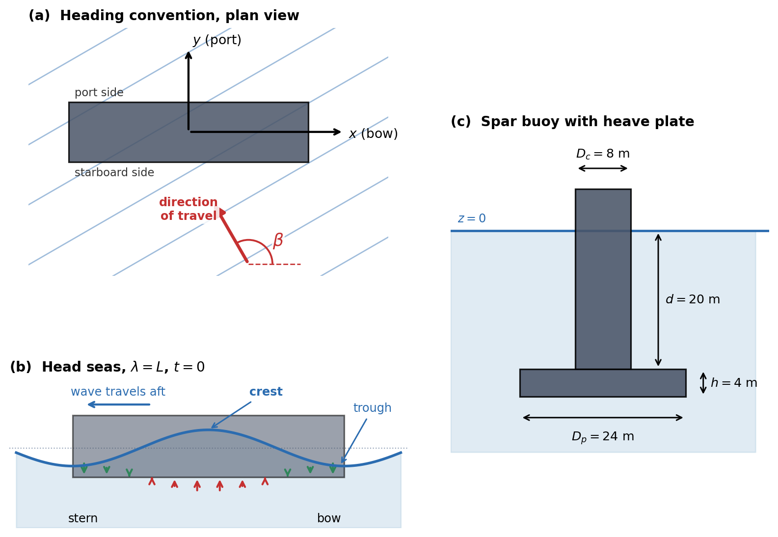
The third is a spar buoy with a heave plate: a vertical circular column of diameter \(D_c = 8\) m, piercing the free surface and extending down to \(z = -20\) m, where it stands on a coaxial circular disc of diameter \(D_p = 24\) m and thickness \(h = 4\) m, so that the disc occupies \(-24 \le z \le -20\) m. It appears only in Problem 7.
Figure 7.1 shows the heading convention on the barge, the head sea case of Problem 4, and the buoy.
Reading the incident wave. The barge lies at rest (\(U = 0\)) in a regular wave of amplitude \(A = 1\) m.
- For each of \(\beta = 0^{\circ}, 45^{\circ}, 90^{\circ}, 135^{\circ}, 180^{\circ}, 225^{\circ}, 270^{\circ}, 315^{\circ}\), give the direction of travel as a unit vector in the BCS and say from which side of the barge the wave arrives (ahead, astern, port, starboard, or one of the four quarters). Two of these are routinely got backwards. Which two, and what is the misreading?
- Head seas, \(\lambda = L = 120\) m. Find \(\omega\), the wave period and the phase speed. At \(t = 0\) a crest stands at \(O\): where are the crests and troughs along the barge at that instant? Where is that crest a quarter of a period later? Confirm from \(\eta^{(1)}\) that it has moved the way \(\beta\) says it should.
- In the same wave, evaluate the total pressure (hydrostatic plus first order dynamic) at the keel amidships, \(z = -8\) m, with the crest overhead and half a period later with the trough overhead. A student argues that the pressure there is simply the hydrostatic head of the local water column, \(\rho g(T + \eta)\). Compare the two, say which is right, and explain the difference from the vertical momentum balance of the fluid under a crest.
- Linear theory integrates the pressure over \(S_{B0}\), which stops at \(z = 0\), even when a crest stands \(1\) m up the side of the barge. Estimate the force on the strip of side between \(z = 0\) and \(z = \eta\), show that it is of second order in \(A\), and say why the strip on the crest side and the strip on the trough side of the barge in beam seas do not cancel on average.
- Show that for any hull that is symmetric about the plane \(y = 0\), the Froude–Krylov loads at heading \(-\beta\) (that is, \(360^{\circ} - \beta\)) are related to those at \(\beta\) by: surge, heave and pitch unchanged; sway, roll and yaw reversed in sign. Argue from how \(\Psi\), \(\hat{n}^{(0)}\) and \(\vec{r}_P^{(0)}\times\hat{n}^{(0)}\) transform under the reflection \(y \rightarrow -y\), then check the claim on the barge summary formulas. Does the same hold for the scattering loads? What does it save the person running the diffraction code?
Three waves, one encounter frequency. The KCS steams at its service speed, \(U = 12.35\) m/s, in deep water.
- For a wave with \(\lambda = L_{pp} = 230\) m, find \(\omega\) and \(T_w\), and then \(\omega_e\) and the encounter period \(T_e\) in head seas and in following seas.
- In following seas, show that \(\omega_e\) has a maximum at \(\omega = g/(2U)\), with value \(g/(4U)\), and find that wave’s length and period. Find also the wave frequency at which \(\omega_e = 0\), show that it is the wave whose phase speed equals \(U\), and describe what the crew sees.
- Still in following seas, find every wave frequency that the ship meets at an encounter period of \(2\pi/0.15 \approx 41.9\) s (that is, \(|\omega_e| = 0.15\) rad/s). Give the wavelength of each, say whether the ship overtakes the wave or the wave overtakes the ship, and say from which end the crests appear to arrive as seen from the bridge.
- Estimate the roll natural period from \(GM_T = 0.60\) m, the roll inertia given above and a roll added inertia of \(15\%\). At \(24\) kn, find the wave periods that meet the ship at this encounter period in head seas (\(\beta = 180^{\circ}\)), beam seas (\(90^{\circ}\)) and stern quartering seas (\(45^{\circ}\)). Which of them lie in the \(5\)–\(20\) s band that carries most of the energy of the sea? Following seas (\(\beta = 0^{\circ}\)) also admit solutions; explain why they can be set aside for roll resonance in a linear analysis.
- An engineer proposes to tabulate every response of the ship against \(\omega_e\) “because the ship oscillates at \(\omega_e\)”. Say which quantities in the problem are naturally functions of \(\omega_e\) and which are naturally functions of \(\omega\) (with \(\beta\) and \(U\)), and explain why a response plotted against \(\omega_e\) in following seas cannot be a function at all.
The Froude–Krylov load does not know the ship is moving. The explorer of this chapter asserts that the Froude–Krylov curves for the three speeds lie exactly on top of one another when plotted against \(\omega\). This problem asks you to prove it, and to find out why the same is not true of the scattering load.
- Let \((x_0, y, z)\) be fixed to the earth, and let the BCS origin move along \(+x_0\) at speed \(U\), so that \(x_0 = x + Ut\). Start from the zero speed incident potential, written in \((x_0, y, z)\) with time factor \(e^{i\omega t}\), and substitute. Show that the time factor becomes \(e^{i\omega_e t}\), and state the amplitude of the potential in the moving frame. Explain why no other amplitude is possible.
- Apply the operator \((i\omega_e - U\,\partial/\partial x)\) of \(\eqref{eq-incident-force-ft}\) to your \(\hat\varphi_I^{(1)}\) and show that the result is exactly \(i\omega\,\hat\varphi_I^{(1)}\). Interpret the operator physically, deduce the pressure on \(S_{B0}\), and conclude that \(\hat{\tau}_I(\omega_e; U) = \hat{\tau}_I(\omega; 0)\) for every mode, heading and speed.
- Using (b), explain why the Froude–Krylov curves of the explorer coincide on the \(\omega\) axis and separate on the \(\omega_e\) axis. For the KCS in head seas with \(\lambda = L_{pp}\), state precisely what is the same and what is different between the Froude–Krylov heave force time histories at \(U = 0\) and at \(24\) kn.
- Suppose the moving frame amplitude were written \(igA/\omega_e\) instead, on the grounds that the ship “sees” \(\omega_e\). Show that every Froude–Krylov load would then be multiplied by \(\omega/\omega_e\). Evaluate that factor for the KCS at \(24\) kn with \(\lambda = L_{pp}\) in head and in following seas, and identify the wave for which the prediction becomes absurd. What general check on any forward speed formula does this suggest?
- The scattering load genuinely depends on \(U\). Point to every place where \(U\) enters the scattering problem and its pressure integral, and explain why the step that made (b) work for \(\hat\varphi_I^{(1)}\) cannot be repeated for \(\hat\varphi_S^{(1)}\).
Heave and pitch of the box barge in head seas. The barge lies at rest in head seas, \(\beta = 180^{\circ}\), with \(A = 1\) m.
- From the summary formulas, show that in head seas \(\hat F_{I3}^{(1)}\) is real, \(\hat F_{I1}^{(1)}\) and \(\hat M_{I2}^{(1)}\) are purely imaginary, and the other three vanish. Say what “real” and “purely imaginary” mean for the timing of each load relative to the crest passing \(O\).
- Tabulate \(\hat F_{I3}^{(1)}\), \(\hat F_{I3}^{(1)}/(\rho g A A_{WP})\) and \(|\hat M_{I2}^{(1)}|\) for \(\lambda/L = 0.5, 0.75, 1, 1.5, 2, 4\) and in the limit \(\lambda/L \rightarrow \infty\). Interpret the sign of \(\hat F_{I3}^{(1)}\) at \(\lambda/L = 0.75\).
- At \(\lambda = L\) (and at \(\lambda = L/2\)) both the heave and the surge force vanish. Explain why from the picture in Figure 7.1(b), not from the algebra. At \(t = 0\), with the crest at midship, the pitch moment is also zero. Is the barge then unloaded? Describe the pressure on the bottom, name the structural load it produces in the hull girder, and estimate the contribution of the bottom pressure to it at the midship section.
- The zeros of the pitch moment are not at \(\lambda = L/n\). Find the two longest wavelengths at which \(\hat M_{I2}^{(1)} = 0\), and the wavelength at which \(|\hat M_{I2}^{(1)}|\) is largest. Explain why weighting the pressure by the lever arm moves the zeros, and compare the location of the maximum with the “\(\lambda \approx 1.5\,L_{pp}\)” quoted for the KCS above.
- Take \(\lambda = 2L\). Before computing, predict the sign of the surge force and of the pitch moment a quarter period after the crest passes \(O\), from where the water is high and where it is low at that instant. Then evaluate \(F_{I1}(t)\), \(F_{I3}(t)\) and \(M_{I2}(t)\) at \(t = 0\) and \(t = T_w/4\) and confirm your prediction.
The Froude–Krylov force is a volume integral in disguise. Let \(V\) be the mean submerged volume of a hull, closed at the top by its waterplane area \(A_{WP}\) in the plane \(z = 0\). The incident wave does not know the body is there, so the incident wave pressure \(\hat p_I\) is smooth everywhere inside \(V\).
With the chapter’s convention that \(\hat{n}^{(0)}\) points into the body, use the divergence theorem to show that \[\hat{\vec{F}}_I = \hat{k}\iint_{A_{WP}}\hat p_I\,dA - \iiint_V \nabla\hat p_I\,dV, \qquad \hat{\vec{M}}_I = \iint_{A_{WP}}\hat p_I\,(\vec{r}\times\hat{k})\,dA - \iiint_V \vec{r}\times\nabla\hat p_I\,dV\] where \(\hat{k}\) is the unit vector along \(+z\). Then use the linearised Euler equation to show that the horizontal Froude–Krylov force is exactly \(\rho\iiint_V \vec{a}_h\,dV\), where \(\vec{a}_h\) is the horizontal acceleration the water would have had if the body were not there. Interpret the extra waterplane term in the vertical.
Rederive the barge heave force \(\rho g A e^{-kT}J_xJ_y\) from (a) in two lines. Then show, for any hull, that in long waves \(\hat F_{I3} \rightarrow \rho g A A_{WP}\) and \((\hat F_{I1}, \hat F_{I2}) \rightarrow i\rho g A k\nabla(\cos\beta, \sin\beta)\).
Prove that in beam seas the Froude–Krylov surge force is zero for any hull at any wavelength, symmetric or not. The HydRA run for the KCS (\(\beta = 90^{\circ}\), \(U = 0\)) gives, per unit \(\rho g A\) in m\(^2\):
\(\omega\) (rad/s) 0.03 0.15 0.30 FK surge \(0.6845\) \(0.7146\) \(0.8079\) FK sway \(1.678 + 4.744i\) \(1.655 + 117.3i\) \(1.585 + 452.7i\) scattering surge \(-0.1971 - 0.0108i\) \(-4.930 - 0.322i\) \(-21.60 - 1.219i\) Explain the small, almost constant, non-zero FK surge and the constant real part of the FK sway. Explain why the scattering surge escapes your proof.
In the same beam seas the KCS shows large Froude–Krylov pitch and yaw moments, which the barge does not have at all. From (a), show that in long beam waves \(\hat M_{I2} \rightarrow -\rho g A A_{WP}\,x_F\) and \(\hat M_{I3} \rightarrow i\rho g A k\nabla x_B\), where \(x_F\) and \(x_B\) are the longitudinal positions of the centre of flotation and the centre of buoyancy. HydRA gives \(\hat F_{I3}/\rho g A = 6135\) m\(^2\) and \(\hat M_{I2}/\rho g A = 7.841\times10^{4}\) m\(^3\) at \(\omega = 0.03\) rad/s, and \(\hat M_{I3}/\rho g A = -178.8 - 415.9i\) m\(^3\) at \(\omega = 0.15\) rad/s. Deduce \(x_F\) and \(x_B\), and compare \(x_B\) with the published \(LCB = -1.48\%\,L_{pp}\).
For the barge in oblique long waves, expand (a) to second order in \(k\) and show that \(\hat M_{I3} \approx \rho g A\,k^2\,\tfrac12\sin 2\beta\left(\iiint_V x^2\,dV - \iiint_V y^2\,dV\right) = \rho g A\,T k^2 LB(L^2 - B^2)\sin 2\beta/24\). Explain why heave starts at order \(k^0\), sway and roll at order \(k\), and yaw only at order \(k^2\). A square barge has no yaw moment at this order. Is that true at every wavelength? Check a \(60\times60\times8\) m barge at \(\lambda = 60\) m for \(\beta = 30^{\circ}\) and \(\beta = 45^{\circ}\), and explain the difference.
In long waves a ship rides the wave — if you take moments about the right point. The barge lies at rest in very long beam seas (\(\beta = 90^{\circ}\), \(kB \ll 1\), \(kT \ll 1\)), with \(KG = 10\) m so that \(z_G = +2\) m. Ignore the radiation and scattering loads for now; part (e) asks why that is legitimate here.
- From the barge summary formulas, obtain the leading order forms of \(\hat F_{I2}\), \(\hat F_{I3}\) and \(\hat M_{I1}\) as \(k \rightarrow 0\), and show that \(\hat M_{I1} \approx -i\rho g A k\nabla z_M\), where \(z_M = z_B + BM_T\) is the height of the transverse metacentre above \(O\).
- Show that, to this order, the Froude–Krylov load is exactly the static buoyancy \(\rho g\nabla\) tilted to be perpendicular to the local water surface, plus the extra lift \(\rho g A A_{WP}\), with the tilted part acting along a line through the metacentre \(M\). Explain why \(M\), and not \(B\), is the right point.
- A student solves the roll equation on its own, \(C_{44}\hat\xi_4 = \hat M_{I1}\) with \(C_{44} = \rho g\nabla GM_T\). Show that this gives a roll angle \(z_M/GM_T\) times the slope of the water surface at \(O\), and evaluate the ratio. Do the same for pitch in head seas, and explain why the student would have got away with it there.
- Now write the coupled sway and roll equations about \(O\) with the rigid body mass matrix of Chapter 5 (note \(M_{24} = M_{42} = -mz_G\)), and keep only the leading order in \(k\). Show that \(\hat\xi_4\) equals the slope of the water surface exactly, so the deck stays parallel to the local water surface, and that \(\hat\xi_2 = -iA\) and \(\hat\xi_3 = A\). Show that these are exactly the displacements of a water particle at the surface. State the student’s error in one sentence.
- Explain why radiation and scattering may be dropped in this limit. Treat heave and sway separately, using the relative motion between the barge and the water.
A buoy that feels no heave force. Take the spar buoy of Figure 7.1(c) at zero speed in deep water. Wherever needed, assume \(\lambda \gg D_p\), so that the horizontal variation of the wave across the buoy can be neglected, and check that assumption in part (c).
- Find the heave Froude–Krylov force in the long wave limit. The disc carries almost two thirds of the displaced volume. Why does it contribute nothing to that limit?
- Using Problem 5(a), or the pressure on each horizontal face directly, show that \[\hat F_{I3} = \rho g A\,e^{-kd}\left[A_c - A_p\left(1 - e^{-kh}\right)\right]\] with \(A_c\), \(A_p\) the column and disc plan areas. Find the wave number \(k^*\), the wavelength and the period at which it vanishes. Show that \(k^*\) does not depend on the depth \(d\) of the disc, explain why, and say what \(d\) does control. What happens to the sign of the force above \(k^*\)?
- Check the \(\lambda \gg D_p\) assumption: in a plane wave, the average of \(e^{-ik(x\cos\beta + y\sin\beta)}\) over a disc of radius \(R\) is \(2J_1(kR)/(kR)\). Insert this factor for the column and the disc, recompute \(k^*\) and comment.
- A fixed heave plate in an accelerating flow also feels a scattering force. In the long wave limit, model it as \(A_{33}\hat a_3\), where \(\hat a_3\) is the vertical acceleration of the undisturbed water at the centre of the disc and \(A_{33} \approx \tfrac{8}{3}\rho R_p^3\) is the added mass of a thin disc in unbounded fluid. Add this to (b), find the new period of zero heave force, and compare it with the Froude–Krylov value. At that period, which is larger: the Froude–Krylov force on the disc or its scattering force? What does this say about the Froude–Krylov hypothesis for a heave plate?
- Compute the heave natural period of the buoy using the same \(A_{33}\) and neglecting the column’s added mass. Compare it with the period from (d), explain why a designer would want the two close together, and name the physical effect, ignored throughout this chapter, that makes heave plates even more effective in practice.
What the scattering problem is, and what it is not. This problem is conceptual and needs arithmetic only in part (c).
- On \(S_{B0}\) the full first order body condition says that the normal velocity of the water equals the normal velocity of the hull. Write the total potential as \(\varphi = \varphi_I + \varphi_S + \varphi_R\), where \(\varphi_R\) is the radiation potential of Chapter 6. Show how the body condition splits between \(\varphi_I + \varphi_S\) and \(\varphi_R\). In the scattering problem, what is the body doing? Why is it legitimate to compute the wave load on a body held fixed and the radiation load on a body moving in calm water, and add them? Name the precise property that makes this possible, and the step in the derivation that would break it.
- Two statements a student makes: “the scattered wave is made by the body’s motion, so a body held fixed does not scatter”, and “a body small compared with the wavelength does not scatter, so Froude–Krylov is enough”. Correct the first. Test the second, in the long wave limit, on (i) the heave force on a long ship in head seas and (ii) the horizontal force on a slender vertical circular pile with added mass coefficient \(C_a = 1\). What fraction of the total load does Froude–Krylov give in each case?
- Very short beam waves on the barge: \(\lambda = 10\) m, \(\beta = 90^{\circ}\). Evaluate the Froude–Krylov sway force from the summary formulas. Then estimate the true sway force by assuming that the weather side reflects the wave completely, as a vertical wall would (a standing wave of amplitude \(2A\) against the weather side, still water in the lee). Compare the two in magnitude, and say which side of the hull carries the load in each picture.
- The scattering problem must be solved afresh for every heading; the radiation problem at zero speed is solved once per frequency, whatever the heading. Explain why, from the body conditions. For the KCS run at \(U = 0\) (50 frequencies, 8 headings), how many boundary value problems of each kind are needed at minimum, using Problem 1(e)? At \(U > 0\) the radiation coefficients do depend on \(\beta\): through what quantity?
- \(\hat\varphi_I\) is known in closed form, while \(\hat\varphi_S\) needs a panel code. Of the conditions in the scattering boundary value problem, which one does \(\hat\varphi_I\) fail to satisfy, and why is that the only reason \(\hat\varphi_S\) exists? The Sommerfeld condition is imposed on \(\hat\varphi_S\) but not on \(\hat\varphi_I\) or \(\hat\varphi_D\). Why would imposing it on either of those be wrong?
How big is the scattering? Reading the KCS numbers. The tables below are taken from the HydRA run behind the interactive explorer. Loads are per unit \(\rho g A\), added mass is \(A_{ij}/\rho\) and damping is \(B_{ij}/(\rho\omega)\), all in m\(^2\) or m\(^3\). Use \(\nabla = 51\,715\) m\(^3\) and \(A_{WP} = 6135\) m\(^2\). In every FK sway entry, discard the constant real part of about \(1.7\) m\(^2\); it is the mesh closure residual of Problem 5(c).
Table A — beam seas (\(\beta = 90^{\circ}\)), \(U = 0\), sway:
\(\omega\) (rad/s) FK sway scattering sway \(A_{22}/\rho\) 0.03 \(1.678 + 4.744i\) \(-0.0027 + 4.097i\) \(44\,680\) 0.09 \(1.671 + 42.54i\) \(-0.0253 + 36.91i\) \(45\,100\) 0.15 \(1.655 + 117.3i\) \(-0.0103 + 102.9i\) \(46\,040\) 0.30 \(1.585 + 452.7i\) \(13.78 + 427.5i\) \(52\,010\) Table B — beam seas, \(U = 0\), heave:
\(\omega\) (rad/s) FK heave scattering heave \(A_{33}/\rho\) \(B_{33}/(\rho\omega)\) 0.15 \(6021\) \(-405.1 + 82.66i\) \(176\,800\) \(36\,930\) 0.30 \(5667\) \(-1253 + 760.2i\) \(138\,100\) \(83\,030\) 0.51 \(4796\) \(-1674 + 1932i\) \(70\,850\) \(70\,570\) 0.75 \(3369\) \(-2055 + 2270i\) \(57\,140\) \(37\,600\) Table C — head seas (\(\beta = 180^{\circ}\)):
\(\omega\) (rad/s) mode FK (any \(U\)) scattering, \(U = 0\) scattering, \(24\) kn 0.42 pitch \(-9693 - 2.250\times10^{5}i\) \(3.060\times10^{4} + 7.697\times10^{4}i\) \(3.014\times10^{4} + 4.908\times10^{4}i\) 0.54 heave \(172.9 - 254.2i\) \(-32.59 + 534.5i\) \(-313.4 + 209.2i\) - From Table A, compute the ratio of scattering to Froude–Krylov sway at each frequency and compare it with \(A_{22}/(\rho\nabla)\). Explain the agreement at low frequency, and hence give the effective Morison inertia coefficient \(C_M\) of the KCS in sway.
- Why does the agreement deteriorate by \(\omega = 0.30\) rad/s? Quote the two non-dimensional numbers that measure the failure of the assumption behind (a).
- In long waves the scattering problem looks like the radiation problem seen from the body: a fixed body in water rising and falling with \(\eta\) is equivalent to the body moving by \(-\eta\) in still water. Use this to argue that the total heave excitation is approximately \(\left(\rho g A_{WP} - \omega^2A_{33} + i\omega B_{33}\right)A\), and test it against Table B. Where does it work and why does it fail?
- From Table C, compute the total pitch moment at \(\omega = 0.42\) rad/s (\(\lambda \approx 1.5\,L_{pp}\)) at both speeds, and the error made by Froude–Krylov alone. Do the same for heave at \(\omega = 0.54\) rad/s. The speed changes the heave scattering only moderately, yet the total heave force changes by a factor of about two. Explain.
- Without the data, which of the six beam sea loads on the KCS would you expect Froude–Krylov to misrepresent most badly, relative to its own size? Use Problem 5(d) to say why.
Programming Problem: Froude–Krylov loads on any hull by panel integration. The Froude–Krylov integrals \(\eqref{eq-incident-force-ft}\) need only the known incident pressure and the geometry of \(S_{B0}\), so they can be evaluated for any hull without solving a boundary value problem.
- Write a function that takes a list of flat panels (centroid \(\vec r_i\), unit normal \(\hat n_i\) pointing into the body, area \(a_i\)), a wave number \(k\) and a heading \(\beta\), and returns the six load amplitudes per unit \(\rho g A\) by the midpoint rule, \(\sum_i\Psi(\vec r_i)\{\hat n_i, \vec r_i\times\hat n_i\}a_i\). Mesh the barge with \(n\times n\) panels on each of its five wetted faces and compare with the closed forms at \(\lambda = L\) for \(\beta = 180^{\circ}\), \(135^{\circ}\), \(90^{\circ}\), for \(n = 5, 10, 20, 40\). Report the error and its order of convergence.
- Mesh the Wigley hull, \(y = \pm\tfrac{B}{2}\left(1 - (2x/L)^2\right)\left(1 - (z/T)^2\right)\), with \(L = 120\) m, \(B = 12\) m, \(T = 7.5\) m, by mapping a grid in \((x, z)\) onto each side. Before computing any loads, verify the mesh: check \(\sum_i\hat n_ia_i\) against \(\hat k A_{WP}\) with \(A_{WP} = \tfrac23LB\), and the displaced volume against \(\nabla = \tfrac49LBT\). Then compute \(\hat F_{I3}\) and \(\hat M_{I2}\) in head seas for \(0.3 \le \lambda/L \le 5\) and confirm the long wave limits of Problem 5(b).
- Plot \(\hat F_{I3}/(\rho g A A_{WP})\) against \(\lambda/L\) for the Wigley hull and for the barge of the same \(L\), \(B\), \(T\). Locate the zeros of each curve. Explain why the Wigley hull’s zeros are not at \(\lambda = L/n\), and why its oscillations at short wavelengths are so much weaker than the barge’s.
- Move the origin to the stern, \(x' = x + L/2\), keeping \(\varepsilon = 0\) at the new origin. Show from the definition of \(\Psi\) that the new loads are \(\hat{\vec F}' = e^{-ik(L/2)\cos\beta}\hat{\vec F}\) and \(\hat{\vec M}' = e^{-ik(L/2)\cos\beta}\left(\hat{\vec M} + \tfrac{L}{2}\hat\imath\times\hat{\vec F}\right)\), and verify both numerically on the Wigley hull at \(\lambda = L\), \(\beta = 135^{\circ}\). Which load magnitudes change, and which do not?
- Your code and HydRA agree on Froude–Krylov loads to a fraction of a percent for the same mesh. State what your code cannot compute, and what would have to be added to it to do so.
Answer Key
Problem 1 — Reading the incident wave
(a) \(\beta\) names where the wave goes; it arrives from the opposite direction.
Directions. The wave travels along \((\cos\beta, \sin\beta)\) and arrives from \(-(\cos\beta, \sin\beta)\): \[{\small\begin{array}{c|c|l|l} \beta & (\cos\beta,\ \sin\beta) & \text{seas} & \text{from} \\ \hline 0^\circ & (+1.00,\ +0.00) & \text{following} & \text{astern} \\ 45^\circ & (+0.71,\ +0.71) & \text{stern quartering} & \text{starboard quarter} \\ 90^\circ & (+0.00,\ +1.00) & \text{beam} & \text{starboard} \\ 135^\circ & (-0.71,\ +0.71) & \text{bow quartering} & \text{starboard bow} \\ 180^\circ & (-1.00,\ +0.00) & \text{head} & \text{ahead} \\ 225^\circ & (-0.71,\ -0.71) & \text{bow quartering} & \text{port bow} \\ 270^\circ & (+0.00,\ -1.00) & \text{beam} & \text{port} \\ 315^\circ & (+0.71,\ -0.71) & \text{stern quartering} & \text{port quarter} \end{array}}\]
The two usually got backwards. \(\beta = 90^\circ\) travels towards port, so it strikes the starboard side first; reading it as a sea on the port side reverses the sign of every lateral load. \(\beta = 0^\circ\) travels the way the bow points, overtaking from astern: following, not head, seas.
Why. Both slips come from naming a wind by where it comes from.
(b) In head seas the crests run aft along the barge.
Wave. \(k = 2\pi/120 = 0.05236\) m\(^{-1}\), \(\omega = \sqrt{gk} = 0.7167\) rad/s, \(T_w = 8.767\) s, \(c = \omega/k = 13.688\) m/s.
At \(t = 0\). With \(\beta = \pi\), \(\eta^{(1)} = A\cos(kx + \omega t)\), i.e. \(A\cos kx\): a crest at \(x = 0\), troughs at \(x = \pm60\) m (bow and stern), next crests at \(\pm120\) m.
A quarter period later. \(\eta^{(1)} = A\cos(kx + \pi/2)\), crest at \(x = -\lambda/4 = -30\) m: the crest has moved aft, as \(\beta = 180^\circ\) says. (\(\cos(kx + \omega t)\) is constant along \(x = -ct\).) A crest takes \(L/c = 8.767\) s, one period, to pass from bow to stern.
(c) The keel feels only a fraction \(e^{-kT}\) of the head of water above it, because the water under a crest is accelerating downwards.
Linear pressure. \(\hat p = \rho gAe^{kz}e^{-ik(x\cos\beta + y\sin\beta)}\), amplitude \(\rho gAe^{-kT}\) at the keel with \(e^{-kT} = 0.6578\). Total: \(87.06\) kPa under the crest, \(73.83\) kPa under the trough.
Water-column guess. \(\rho g(T \pm A) = 90.50\) and \(70.39\) kPa: the fluctuation is overstated by \(e^{kT} = 1.520\): the keel feels only \(66\%\) of the head of water above it. The linear result is right.
Why. Hydrostatics assumes no acceleration. Under a crest the particles are at the top of their orbits, accelerating downwards with \(a_z = -\omega^2Ae^{kz}\), and \(\partial p/\partial z = -\rho(g + a_z)\) makes the pressure grow more slowly than hydrostatic, as if gravity were reduced. Integrating to the keel gives exactly \(e^{-kT}\), which is why deep hulls feel so little of short waves (figure below).

(d) The force on the strip above \(z = 0\) is second order, and its mean does not cancel: it is the origin of the wave drift force.
Size. Between \(z = 0\) and \(z = \eta\) the pressure is nearly hydrostatic, \(\rho g(\eta - z)\), giving \(\tfrac12\rho g\eta^2\) per unit length: pressure (\(\propto A\)) times height (\(\propto A\)), so \(O(A^2)\). Over \(120\) m with \(A = 1\) m, about \(0.60\) MN, against a first order sway amplitude of \(11.2\) MN in beam seas; halving \(A\) quarters the first and halves the second.
Why the two sides do not cancel. \(\eta^2 \ge 0\), so each strip pushes inwards whenever it is wetted, and the weather side, seeing incident and reflected wave, is wetted more. The difference has a non-zero mean: the mean wave drift force, invisible to linear theory.
(e) Reflecting the heading across the centreline leaves surge, heave and pitch unchanged and reverses sway, roll and yaw, for Froude–Krylov and scattering alike.
Pressure. The reflection \(R: y \to -y\) maps the symmetric hull onto itself, and \(\Psi(x, -y, z; -\beta) = \Psi(x, y, z; \beta)\), so the mirror panel at \(-\beta\) sees the pressure the original panel sees at \(\beta\).
Geometry. The normal reflects as \((n_1, -n_2, n_3)\); the lever \(\vec r\times\hat n\) picks up \(\det R = -1\) and transforms as \((-m_1, m_2, -m_3)\). Summing over mirror pairs, \(F_1, F_3, M_2\) are unchanged and \(F_2, M_1, M_3\) change sign.
Check on the barge (\(\lambda = 120\) m): \(\hat\tau_{Ij}(-135^\circ)/\hat\tau_{Ij}(135^\circ) = (+1.0000, -1.0000, +1.0000, -1.0000, +1.0000, -1.0000)\).
Scattering. The same holds: Laplace’s equation, the free surface, bottom and radiation conditions, the hull and the forward speed along \(x\) are all unchanged by \(R\), and the body condition is driven by \(\partial\hat\varphi_I/\partial n\), which reflects as above.
Saving. Only headings \(0^\circ\)–\(180^\circ\) need solving: \(225^\circ\), \(270^\circ\) and \(315^\circ\) of the KCS run follow from \(135^\circ\), \(90^\circ\) and \(45^\circ\), three eighths of the work.
Problem 2 — Three waves, one encounter frequency
(a) The same wave is met about five times more often heading into it than running before it.
Wave. \(k = 2\pi/230 = 0.02732\) m\(^{-1}\), \(\omega = 0.5177\) rad/s, \(T_w = 12.14\) s; Doppler term \(\omega^2U/g = 0.3374\) rad/s.
Head seas. \(\omega_e = \omega + \omega^2U/g = 0.8551\) rad/s, \(T_e = 7.35\) s.
Following seas. \(\omega_e = \omega - \omega^2U/g = 0.1803\) rad/s, \(T_e = 34.8\) s.
(b) In following seas the encounter frequency has a ceiling, and the wave that moves at the ship’s speed stands still relative to it.
Maximum. \(d\omega_e/d\omega = 1 - 2\omega U/g = 0\) at \(\omega^* = g/(2U) = 0.3972\) rad/s, where \(\omega_e = g/(4U) = 0.1986\) rad/s (\(T_e = 31.6\) s); that wave has \(\lambda = 391\) m and \(T_w = 15.82\) s. No following wave is met more often than every \(31.6\) s.
Zero. \(\omega_e = 0\) at \(\omega_0 = g/U = 0.7943\) rad/s (\(\lambda = 97.7\) m, \(T_w = 7.91\) s), where \(c = g/\omega = U\).
What the crew sees. A frozen wave: the same crest stays at the same place along the hull, the load is constant, and a crest amidships can hold the ship on its reduced stability for a long time: a route to capsize, surf-riding and broaching.
(c) Three very different waves are all met once every \(42\) s.
Roots. With \(a = U/g = 1.25892\) s: \(\omega_e = +0.15\) gives \(a\omega^2 - \omega + 0.15 = 0\), two roots (since \(0.15 < g/4U\)); \(\omega_e = -0.15\) gives \(a\omega^2 - \omega - 0.15 = 0\), one positive root.
\[\begin{array}{c|c|c|c|c|l} \omega\ \text{(rad/s)} & T_w\ \text{(s)} & \lambda\ \text{(m)} & \omega_e & c\ \text{(m/s)} & \text{seen from} \\ \hline 0.2007 & 31.30 & 1530 & +0.1500 & 48.87 & \text{astern} \\ 0.5936 & 10.58 & 175 & +0.1500 & 16.53 & \text{astern} \\ 0.9234 & 6.80 & 72 & -0.1500 & 10.62 & \text{ahead} \end{array}\]
Reading. A 1530 m swell, an ordinary 175 m sea and a 72 m chop. The first two are faster than the ship (\(c > U = 12.35\) m/s) and overtake it; the third is slower, so its crests appear to come from ahead, as the negative \(\omega_e\) records.
(d) Only in stern quartering seas does an energetic wave meet the ship at its roll natural period, and forward speed is what makes it possible.
Roll period. \(C_{44} = \rho g\nabla GM_T = 3.1201 \times 10^{8}\) N·m/rad, \(I_{44} + A_{44} = 1.15\times9.4614 \times 10^{9} = 1.0881 \times 10^{10}\) kg·m\(^2\), so \(T_4 = 37.1\) s and \(\omega_4 = 0.1693\) rad/s.
Waves met at \(T_e = T_4\). \[\begin{array}{c|l} \beta & T_w\ \text{(s)} \\ \hline 180^\circ & 43.8 \\ 90^\circ & 37.1 \\ 45^\circ & 30.2,\ 6.9,\ 4.9 \\ 0^\circ & 25.7,\ 11.4,\ 6.7 \end{array}\]
Which are in the band. Head seas need a very long swell and beam seas a \(37\) s wave: neither in \(5\)–\(20\) s. Stern quartering seas give a \(6.9\) s wave, squarely in the band.
Following seas. Set aside because the first order roll moment at \(\beta = 0^\circ\) is zero by symmetry (Problem 1(e)). (Parametric roll, by modulation of \(GM_T\), is nonlinear and outside this chapter.) (Figure below.)

(e) Dynamics belong to \(\omega_e\); excitation belongs to \(\omega\) and \(\beta\). Against \(\omega_e\), a following-sea response is not even a function.
Functions of \(\omega_e\). Everything describing the body’s own dynamics: \(-\omega_e^2(\boldsymbol{M} + \boldsymbol{A})\), \(i\omega_e\boldsymbol{B}\), and \(\boldsymbol{A}\), \(\boldsymbol{B}\) themselves (with \(U\) as a parameter).
Functions of \(\omega\) and \(\beta\). The excitation: its spatial structure \(e^{kz}e^{-ik(x\cos\beta + y\sin\beta)}\) is set by \(k = \omega^2/g\).
Not a function. Part (c) gives three wavelengths, three pressure distributions and three excitations at one \(\omega_e\): a response plotted against \(\omega_e\) takes three values at one abscissa and cannot be interpolated or integrated against a spectrum. Responses are therefore tabulated against \(\omega\) for each \(\beta\) and \(U\). The same fold makes the encounter spectrum \(S_e(\omega_e) = S(\omega)/|d\omega_e/d\omega|\) singular (integrably) at \(\omega = g/(2U)\).
Problem 3 — The Froude–Krylov load does not know the ship is moving
(a) Changing to the moving frame relabels the points but cannot rescale the wave: the amplitude keeps \(\omega\), not \(\omega_e\).
Substitution. With \(x_0 = x + Ut\), \[\begin{aligned} e^{-ik(x_0\cos\beta + y\sin\beta) + i\omega t} &= e^{-ik(x\cos\beta + y\sin\beta)}\,e^{i(\omega - kU\cos\beta)t} \\ &= e^{-ik(x\cos\beta + y\sin\beta) + i\omega_et}, \end{aligned}\] so the time factor is \(e^{i\omega_et}\) with \(\omega_e = \omega - kU\cos\beta\).
Amplitude. Unchanged: \[\hat\varphi_I^{(1)} = \frac{igA}{\omega}\,e^{kz}\,e^{-ik(x\cos\beta + y\sin\beta) + i\varepsilon}.\]
Why no other. The potential at a point of the water at an instant is a fact about the water, not the observer: same particle velocities, same pressures, with or without a ship steaming through.
(b) The pressure operator is the time derivative at a point fixed in the earth, which for an incident wave is just \(i\omega\).
Operator. \(\partial/\partial x\) on a plane wave is multiplication by \(-ik\cos\beta\), so \[\left(i\omega_e - U\frac{\partial}{\partial x}\right)\hat\varphi_I^{(1)} = \left(i\omega_e + ikU\cos\beta\right)\hat\varphi_I^{(1)} = i\omega\,\hat\varphi_I^{(1)}.\]
Meaning. A point fixed in the earth moves at \(-U\) relative to the BCS, so \(\partial_t|_{\text{earth}} = \partial_t|_{\text{ship}} - U\partial_x\); Bernoulli needs the derivative following the water.
Consequence. \[\hat p_I = -\rho\,i\omega\,\hat\varphi_I^{(1)} = \rho gA\,e^{kz}\,e^{-ik(x\cos\beta + y\sin\beta) + i\varepsilon},\] the zero speed pressure on a speed-independent \(S_{B0}\): \(\hat\tau_I(\omega_e; U) = \hat\tau_I(\omega; 0)\) for every mode, heading and speed.
(c) Against \(\omega\) the curves coincide; against \(\omega_e\) the same values are only relabelled.
Why. Each speed gives the same \(\hat\tau_I(\omega; 0)\); plotting against \(\omega_e\) stretches head-sea curves to higher \(\omega_e\) and folds following-sea curves back (Problem 2). Nothing happens to the load.
KCS, head seas, \(\lambda = L_{pp}\). Same amplitude and same phase relative to the crest at \(O\); different period, \(12.14\) s at rest and \(7.35\) s at \(24\) kn, because the crests are met \(1.65\) times as often (figure below).

(d) A \(1/\omega_e\) in a wave quantity fails Galilean invariance and blows up when the ship rides a crest.
Factor. With \(igA/\omega_e\), \(-\rho\,i\omega\cdot igA/\omega_e = \rho gA(\omega/\omega_e)\): every load is multiplied by \(\omega/\omega_e\).
KCS at \(24\) kn, \(\lambda = L_{pp}\). Head seas \(\omega/\omega_e = 0.5177/0.8551 = 0.605\), a load 39% too small; following seas \(\omega/\omega_e = 0.5177/0.1803 = 2.87\), 2.9 times too large.
Absurd. At \(\omega = g/U = 0.7943\) rad/s (\(\lambda = 98\) m), \(\omega_e = 0\) and the factor is infinite: ordinary water at ordinary pressure would exert an infinite force.
General check. Galilean invariance: anything belonging to the undisturbed wave must be independent of the observer’s speed and stay finite as \(\omega_e \to 0\).
(e) The scattered field is not one plane wave, so the Doppler shift cannot be absorbed into a single frequency.
Where \(U\) enters. The free surface condition \(\left(i\omega_e - U\partial_x\right)^2\hat\varphi_S^{(1)} + g\,\partial_z\hat\varphi_S^{(1)} = 0\); the pressure operator of \(\eqref{eq-scattering-force-ft}\); and, through \(\omega_e\), the radiation condition. (The body condition is speed independent by (a).)
Why (b) cannot be repeated. It worked because \(\hat\varphi_I\) is a single plane wave. \(\hat\varphi_S\) spreads from the hull in every direction, a superposition of all directions, each Doppler-shifted differently: waves scattered forward are compressed, those scattered aft stretched. The scattering load therefore depends on \(U\) even on the \(\omega\) axis, as the explorer shows. (A complete theory adds further \(U\) dependence from the steady flow round the hull.)
Problem 4 — Heave and pitch of the box barge in head seas
(a) Heave responds to the height of the wave and peaks with the crest at midship; surge and pitch respond to its slope and peak a quarter period later.
Head seas. \(\beta = \pi\): \(u = -kL/2\), \(v = 0\), \(J_y = B\), \(L_y = 0\), \(\sin v = 0\), so \(\hat F_{I2} = \hat M_{I1} = \hat M_{I3} = 0\).
Real and imaginary. \(\hat F_{I3} = \rho gAe^{-kT}J_xB\) is real. \(\hat F_{I1} = 2i\rho gAJ_zB\sin u\) and \(\hat M_{I2} = \rho gAB(-e^{-kT}L_x + 2iK_z\sin u)\) (with \(L_x\) itself \(i\) times a real number) are purely imaginary.
Timing. With \(\tau(t) = \operatorname{Re}\{\hat\tau e^{i\omega t}\}\), a real amplitude gives \(\cos\omega t\), extreme as the crest passes \(O\); an imaginary one gives \(\sin\omega t\), extreme a quarter period later, when \(O\) is on a node and the surface slope at midship is greatest.
(b) In long waves the barge is lifted by the whole waterplane; at \(\lambda/L = 0.75\) it is pushed down while the crest is at midship.
Table (\(\hat F_{I3}/\rho gA\) in m\(^2\), \(|\hat M_{I2}|/\rho gA\) in \(10^3\) m\(^3\); multiply by \(\rho g = 10055\) N/m\(^3\) for newtons): \[\begin{array}{c|c|c|c} \lambda/L & \hat F_{I3}/\rho gA & \hat F_{I3}/(\rho gAA_{WP}) & |\hat M_{I2}|/\rho gA \\ \hline 0.5 & 0 & 0 & 14.87 \\ 0.75 & -425.8 & -0.1183 & 9.81 \\ 1 & 0 & 0 & 45.23 \\ 1.5 & +1125.9 & +0.3127 & 69.87 \\ 2 & +1858.8 & +0.5163 & 69.33 \\ 4 & +2918.9 & +0.8108 & 46.59 \\ \infty & +3600 & +1.0000 & 0 \end{array}\]
Long waves. \(\hat F_{I3} \to \rho gAA_{WP}\): the restoring force \(C_{33}\) times a sea rising uniformly under the barge.
Negative at \(0.75\). With a crest at midship the bottom spans one crest and parts of two troughs, and the troughs win: the barge is pushed down while the water at midship is highest. The phase describes the pressure averaged over the bottom, not the local wave.
(c) No heave force does not mean no load: at \(\lambda = L\) the bottom pressure bends the hull girder hardest.
Why the forces vanish. The bottom spans exactly one wavelength and carries equal areas of positive and negative pressure at every instant; the bow and stern faces, a wavelength apart, see equal and opposite pressures (\(\sin(kL/2) = \sin\pi = 0\); likewise \(\sin 2\pi = 0\) at \(\lambda = L/2\)).
Not unloaded. At \(t = 0\) the bottom pressure \(\rho gAe^{-kT}\cos kx\) pushes up amidships and down at both ends: a beam pushed up in the middle, hogging, the vertical wave bending moment. Half a period later it is sagging.
Estimate. Moments about midship of the pressure on the forward half (which has no net force): \[M_{\text{bend}} = \rho gAe^{-kT}B\left|\int_0^{L/2}x\cos kx\,dx\right| = \frac{2\rho gAe^{-kT}B}{k^2},\] \(145\) MN·m per metre of amplitude: why \(\lambda \approx L\) is the design wave for longitudinal strength (figure below).
(d) The pitch moment needs zero first moment of pressure to vanish, a different condition from zero mean, so its zeros move.
Numbers. Zeros at \(\lambda/L = 0.691\) and \(0.401\); maximum at \(\lambda/L = 1.69\) with \(|\hat M_{I2}|/\rho gA = 71.0\times10^3\) m\(^3\).
Why the zeros move. \(\int x\sin kx\,dx = 0\) over \([-L/2, L/2]\) gives \(\tan(kL/2) = kL/2\), not \(\sin(kL/2) = 0\); the end-face term \(2iK_z\sin u\) shifts the roots a little more.
Why the maximum is above \(\lambda = L\). A moment needs bow and stern on opposite slopes (\(\lambda\) comparable with \(L\)), while the slope \(kA\) falls as \(\lambda\) grows. The compromise is \(\lambda \approx 1.7L\) here, near \(1.5\,L_{pp}\) for the KCS, whose fine ends shorten its effective length.

(e) A quarter period after the crest passes, the water is low forward and high aft: the barge is pushed forward and pitched bow down.
Prediction. At \(t = T_w/4\), \(\eta = -A\sin kx\): low forward, high aft. The stern face carries more pressure than the bow face, so \(F_{I1} > 0\); the bottom has extra buoyancy aft, so the stern rises and the bow drops: a positive (bow-down) pitch moment.
Check at \(\lambda = 2L\), with \(\hat F_{I1} = -4.355i\) MN, \(\hat F_{I3} = 18.69\) MN, \(\hat M_{I2} = -697.1i\) MN·m: \[\begin{array}{c|c|c|c} & F_{I1}\ \text{(MN)} & F_{I3}\ \text{(MN)} & M_{I2}\ \text{(MN·m)} \\ \hline t = 0 & +0.000 & +18.690 & +0.000 \\ t = T_w/4 & +4.355 & +0.000 & +697.107 \end{array}\]
Verdict. Both signs as predicted, and the heave force passes through zero as the crest leaves midship. Since \(\operatorname{Re}\{\hat\tau e^{i\pi/2}\} = -\operatorname{Im}\hat\tau\), predicting physically and checking against \(-\operatorname{Im}\hat\tau\) is the quickest test of a sign convention.
Problem 5 — The Froude–Krylov force is a volume integral in disguise
(a) The Froude–Krylov force is the force that would give the displaced water the acceleration it would have had, plus, vertically, the pressure acting up through the waterplane.
Divergence theorem. Close \(S_{B0}\) with the lid \(A_{WP}\). The outward normal is \(-\hat n^{(0)}\) on \(S_{B0}\) and \(+\hat k\) on the lid, and \(\oint\hat p\,\hat n_{\text{out}}\,dS = \iiint_V\nabla\hat p\,dV\), so \[\iint_{S_{B0}}\hat p\,\hat n^{(0)}dS = -\left(\iiint_V\nabla\hat p\,dV - \iint_{A_{WP}}\hat p\,\hat k\,dA\right).\]
Moment. The \(i\)-th component of \(\oint\hat p(\vec r\times\hat n_{\text{out}})\,dS\) is \(\epsilon_{ijk}\iiint_V(\delta_{jk}\hat p + r_j\partial_k\hat p)\,dV = \iiint_V(\vec r\times\nabla\hat p)_i\,dV\), since \(\epsilon_{ijk}\delta_{jk} = 0\).
Horizontal force. The linearised Euler equation gives \(-\nabla\hat p_I = \rho\hat{\vec a}\), so \(\hat F_{I1,2} = \rho\iiint_V\hat a_{1,2}\,dV\) exactly: the Froude–Krylov hypothesis.
The lid term. The dynamic pressure acting up through the waterplane: the column above \(z = 0\) is not part of \(V\), and its weight changes as crests and troughs pass. A fully submerged body has no lid term.
(b) In long waves only \(A_{WP}\) and \(\nabla\) survive, for any hull.
Barge heave in two lines. With \(\hat p_I = \rho gA\Psi\) and \(\partial_z\Psi = k\Psi\): \(\hat F_{I3}/\rho gA = J_xJ_y - kJ_xJ_yJ_z = J_xJ_y(1 - (1 - e^{-kT})) = e^{-kT}J_xJ_y\).
Long waves. \(\Psi \to 1 - ik(x\cos\beta + y\sin\beta) + kz + O(k^2)\): the lid term is \(A_{WP}\) and the volume term \(O(k)\), so \(\hat F_{I3} \to \rho gAA_{WP}\). Horizontally \(\partial_x\Psi = -ik\cos\beta\,\Psi\), giving \(\hat F_{I1} \to i\rho gAk\nabla\cos\beta\) and \(\hat F_{I2} \to i\rho gAk\nabla\sin\beta\). (Barge, head seas: \(2i\rho gATB\sin(-kL/2) \approx -i\rho gAkLBT\).)
(c) In beam seas the water is not accelerated along \(x\) anywhere, so the Froude–Krylov surge is zero for every hull; the KCS numbers that say otherwise are mesh residuals.
Proof. \(\Psi = e^{kz}e^{-iky}\) has no \(x\) dependence, so \(\partial_x\hat p_I \equiv 0\) in \(V\) and the lid has no \(x\) component: \(\hat F_{I1} = 0\) for any shape and any \(k\).
The KCS residuals. About \(0.7\) m\(^2\) of surge, nearly constant, and a constant real part of about \(1.7\) m\(^2\) in sway: mesh closure errors. As \(k \to 0\), \(\hat F_I/\rho gA \to \iint_{S_{B0}}\hat n\,dS\), which for a closed surface is \(\hat kA_{WP}\) exactly; panels that do not quite close leave a horizontal residual added to every frequency. Checking \(\iint\hat n\,dS = \hat kA_{WP}\) is a standard mesh test.
The scattering surge (about \(-22\) m\(^2\) at \(\omega = 0.3\)) is real: the proof needed \(\hat p_I\) uniform in \(x\), but the scattered field inherits the hull’s shape, and the KCS’s fine bow and broad transom scatter differently. The fore–aft symmetric barge would have none at zero speed; forward speed breaks that symmetry.
(d) The uniform lift of a beam sea acts through the centre of flotation and the uniform sideways push through the centre of buoyancy; off \(O\), each has a lever.
Pitch. With \(\partial_x\hat p = 0\), \(\partial_y\hat p = -ik\hat p\), \(\partial_z\hat p = k\hat p\) and \(\vec r\times\hat k = (y, -x, 0)\): lid \(-\iint x\hat p\,dA\), volume \(k\iiint x\hat p\,dV\), so \(\hat M_{I2} \to \rho gA(-A_{WP}x_F + k\nabla x_B) \to -\rho gAA_{WP}x_F\).
Yaw. No lid term; volume term \(ik\iiint x\hat p\,dV \to i\rho gAk\nabla x_B\).
From the data. \(x_F = -7.841e+04/6135 = -12.78\) m; with \(k = 0.15^2/g = 0.002294\) m\(^{-1}\) and \(\nabla = 51715\) m\(^3\), \(x_B = -415.9/(k\nabla) = -3.51\) m, against the published \(-3.40\) m (\(3\%\), about what the dropped \(e^{kz}\) and the mesh account for). The real part, \(-178.8\) m\(^3\), is again a closure residual.
Barge. \(x_F = x_B = 0\), so both moments vanish. The KCS must pitch and yaw in pure beam seas because its centres lie aft of midship.
(e) Each load’s order in \(k\) counts the differences across the hull it needs; yaw needs a difference of a difference.
Expansion. The barge’s first moments and \(xz\), \(yz\) moments vanish, so the first surviving yaw term needs one more factor \(k\) from expanding the exponential: \[\hat M_{I3} \approx \rho gA\,k^2\sin\beta\cos\beta\left(\iiint_Vx^2\,dV - \iiint_Vy^2\,dV\right),\] which with \(\iiint x^2 = BTL^3/12\), \(\iiint y^2 = LTB^3/12\) is \(\rho gA\,Tk^2LB(L^2 - B^2)\sin2\beta/24\). Check at \(\lambda = 5\) km, \(\beta = 30^\circ\): summary \(22.03\) m\(^3\), expansion \(22.15\) m\(^3\).
Orders. Heave: no difference, \(O(1)\). Sway: one side minus the other, \(O(k)\), the slope. Roll: the same difference times a lever, still \(O(k)\). Yaw: the sideways push differing between bow and stern, \(O(k^2)\), the curvature; the crests must be oblique, hence \(\sin2\beta\).
Square barge. The \(k^2\) term vanishes but not the higher ones: at \(\lambda = 60\) m, \(|\hat M_{I3}|/\rho gA = 4389.8\) m\(^3\) at \(30^\circ\) but \(2.5e-12\) m\(^3\) (zero to rounding) at \(45^\circ\). At \(45^\circ\), reflection across the diagonal maps hull and wave onto themselves while reversing the sense of yaw, so the moment vanishes at every wavelength; at \(30^\circ\) there is no such symmetry (figure below).

Problem 6 — In long waves a ship rides the wave — if you take moments about the right point
(a) In long beam waves the sway force is set by the displacement and the roll moment acts about the metacentre.
Limits. With \(\beta = \pi/2\): \(u = 0\), \(J_x = L\), \(L_x = 0\), \(v = kB/2\); for \(k \to 0\), \(\sin v \approx kB/2\), \(J_z \approx T\), \(K_z \approx -T^2/2\), \(e^{-kT} \approx 1\), \(L_y \approx -ikB^3/12\).
Loads. \[\hat F_{I2} \approx 2i\rho gA\,TL\frac{kB}{2} = i\rho gAk\nabla,\] \[\hat F_{I3} \approx \rho gALB = \rho gAA_{WP},\] \[\begin{aligned} \hat M_{I1} &\approx \rho gAL\left(-\frac{ikB^3}{12} - 2i\left(-\frac{T^2}{2}\right)\frac{kB}{2}\right) \\ &= -i\rho gAk\left(I_{yy}^A + \nabla z_B\right) = -i\rho gAk\nabla z_M. \end{aligned}\]
Values. \(z_B = -4.0\) m, \(BM_T = 9.375\) m, \(z_M = 5.375\) m. Check at \(\lambda = 10\) km: \(\hat F_{I2}/(i\rho gAk\nabla) = 0.997476\), \(\hat M_{I1}/(-i\rho gAk\nabla z_M) = 0.993739\).
(b) The long-wave load is buoyancy turned to stay perpendicular to the water, acting through the metacentre.
Tilted buoyancy. The surface \(\eta = Ae^{-iky}\) has slope \(-ikA\) at \(O\); tilting \(\rho g\nabla\hat k\) to the surface normal \(\propto (0, -\partial\eta/\partial y, 1)\) gives a horizontal part \(i\rho gAk\nabla\), exactly \(\hat F_{I2}\).
Line of action. \((0, \hat F_{I2}, 0)\) through \((0, 0, z_M)\) has moment \((-z_M\hat F_{I2}, 0, 0) = (-i\rho gAk\nabla z_M, 0, 0)\), exactly \(\hat M_{I1}\). The extra lift \(\rho gAA_{WP}\) acts at \(y = 0\) and adds no roll moment.
Why \(M\). Tilting the water relative to the hull is, for the underwater shape, the same as tilting the hull relative to the water: \(B\) moves sideways and the new buoyancy vector cuts the centreline at the metacentre. Through \(B\) one would miss the \(I_{yy}^A\) (wedge) part, most of the moment.
(c) Solving roll on its own overstates the roll by \(z_M/GM_T\), a large error when \(GM\) is small and a negligible one in pitch.
Roll alone. \(\hat\xi_4 = \hat M_{I1}/C_{44} = (z_M/GM_T)(-ikA)\), while the angle that keeps the deck parallel to the surface is \(\partial\eta/\partial y = -ikA\). Too large by \(z_M/GM_T = 5.375/3.375 = 1.593\): 59% too much roll.
Pitch alone, head seas. \(z_{M_L}/GM_L = 146.0/144.0 = 1.0139\), only \(1.4\%\).
Why. Both ratios are \(1 + z_G/GM\): large when \(GM\) is small (roll), negligible when \(GM_L = 144\) m (pitch).
(d) With sway–roll coupling kept, the barge moves exactly like a surface water particle and its deck stays parallel to the water.
Equations about \(O\) (\(M_{22} = m\), \(M_{24} = M_{42} = -mz_G\), \(M_{44} = I_{44}\)): \[-\omega^2\left(m\hat\xi_2 - mz_G\hat\xi_4\right) = \hat F_{I2},\] \[-\omega^2\left(-mz_G\hat\xi_2 + I_{44}\hat\xi_4\right) + C_{44}\hat\xi_4 = \hat M_{I1}.\]
Orders. \(\hat F_{I2} = O(k)\) and \(\omega^2 = gk\), so \(\hat\xi_2 = O(1)\) and \(\hat\xi_4 = O(k)\); terms \(\omega^2(\cdot)\hat\xi_4\) are \(O(k^2)\) and drop.
Sway. \(\hat\xi_2 = -\hat F_{I2}/(\omega^2m) = -i\rho gAk\nabla/(gk\rho\nabla) = -iA\).
Roll. The coupling \(\omega^2mz_G\hat\xi_2 = -i\rho gAk\nabla z_G\) is \(O(k)\) and must be kept: \[C_{44}\hat\xi_4 = -i\rho gAk\nabla(z_M - z_G) = -i\rho gAk\nabla\,GM_T,\] \[\hat\xi_4 = -ikA = \frac{\partial\eta}{\partial y}\bigg|_O.\]
Heave. \(\rho gA_{WP}\hat\xi_3 = \hat F_{I3}\), so \(\hat\xi_3 = A\): with \(\hat\xi_2 = -iA\), the circular orbit of a surface particle.
The student’s error. The barge accelerates sideways, and the inertia reaction of that acceleration acts at \(G\), a height \(z_G\) above \(O\), so it has a roll moment about \(O\) that the single roll equation leaves out.
(e) Radiation and scattering drop out because the barge moves with the water: what they depend on is the motion of the water relative to the body.
Heave. The hydrodynamic terms are \((\omega^2A_{33} - i\omega B_{33})\times\)displacement with \(\omega^2 = gk\): \(O(k)\) relative to \(\rho gAA_{WP}\) (Problem 9 confirms on the KCS).
Sway. Here they are of the same order as \(\hat F_{I2}\) but cancel: scattering on the fixed body is \(A_{22}\hat a_2\) (Taylor), radiation on the accelerating body is \(-A_{22}\ddot{\hat\xi}_2\), and their sum depends only on the relative acceleration, which (d) shows is zero. Radiation damping also vanishes as \(\omega \to 0\).
Consequence. A ship in a long swell rides it like a cork; RAOs tend to \(\hat\xi_3/A = 1\) and \(\hat\xi_{4,5}/(kA) = 1\). The interesting cases are where this breaks down: \(\lambda\) comparable with the ship (Problem 4) and encounter near a natural frequency (Problem 2).
Problem 7 — A buoy that feels no heave force
(a) In a very long wave the buoy is lifted only through its waterplane; the submerged disc adds nothing.
Areas and volumes. \(A_c = 50.27\) m\(^2\), \(A_p = 452.39\) m\(^2\); column \(A_cd = 1005.3\) m\(^3\), disc \(A_ph = 1809.6\) m\(^3\), \(64\%\) of \(\nabla = 2814.9\) m\(^3\).
Limit. \(\hat F_{I3} \to \rho gAA_{WP} = \rho gAA_c = 505.4\) kN per metre of amplitude.
Why the disc adds nothing. The long-wave pressure \(\rho gA\) is uniform in depth: it pushes down on the disc’s top annulus and up on its whole underside, netting \(\rho gAA_c\) under the column, as if the column simply continued. A fully submerged volume changes its displacement not at all when the sea rises, just as it added no stiffness in Chapter 6.
(b) The column’s lift and the disc’s downward pull balance at one wavelength, set by the plate’s thickness and the area ratio, not by its depth.
Derivation (Problem 5(a), \(\hat p = \rho gAe^{kz}\)). Lid \(A_c\); column volume \(-A_c(1 - e^{-kd})\); disc \(-A_pe^{-kd}(1 - e^{-kh})\). Sum: \(\hat F_{I3} = \rho gAe^{-kd}\left[A_c - A_p(1 - e^{-kh})\right]\).
Zero. \(1 - e^{-kh} = A_c/A_p\): \[k^* = -\frac{1}{h}\ln\left(1 - \frac{A_c}{A_p}\right) = 0.02945\ \text{m}^{-1},\] \(\lambda^* = 213\) m, \(T^* = 11.69\) s.
Why \(d\) drops out. \(e^{-kd}\) multiplies both competing terms equally: both scale with the local pressure at depth \(d\). What \(d\) controls is the size of the force away from the zero.
Above \(k^*\). The disc wins and the force is \(180^\circ\) out of phase: the buoy is pushed down under a crest, as the water accelerating downward acts on the large disc.
(c) The long-wave assumption is good; finite size only nudges the zero.
Factors at \(k^*\). \(kR_c = 0.1178\), \(kR_p = 0.3533\), so \(2J_1(kR)/(kR) = 0.99827\) (column) and \(0.98447\) (disc).
New zero. \(A_cf_c = A_pf_p(1 - e^{-kh})\) gives \(k^* = 0.02990\) m\(^{-1}\), \(T^* = 11.60\) s, a \(+1.5\%\) shift: the disc spans more of a wavelength than the column, so its term weakens slightly. \(\lambda^* = 213\) m is nine times \(D_p\).
(d) For a thin, wide plate the scattering force dominates the Froude–Krylov force: the plate obstructs far more water than it displaces.
Scattering force. \(\hat a_3 = -\omega^2Ae^{kz}\) (downward under a crest), so \(A_{33}\hat a_3 = -\rho gA(A_{33}/\rho)ke^{-kd_c}\) with \(d_c = d + h/2\): the same sign as the disc’s Froude–Krylov term. \(A_{33}/\rho = \tfrac83R_p^3 = 4608\) m\(^3\), \(2.5\) times the disc’s volume.
New zero. \[\frac{\hat F_{I3} + \hat F_{S3}}{\rho gA} = e^{-kd}\left[A_c - A_p(1 - e^{-kh})\right] - \frac{A_{33}}{\rho}ke^{-kd_c} = 0\] at \(k = 0.00796\) m\(^{-1}\), \(\lambda = 790\) m, \(T = 22.5\) s, against \(T^* = 11.7\) s.
Comparison at that period. Disc Froude–Krylov \(12.09\,\rho gA\), scattering \(30.78\,\rho gA\): 2.5 times larger. The Froude–Krylov hypothesis is the wrong answer here, not a small error (figure below).

(e) The natural period sits close to the period of zero excitation, which removes most of the resonant peak.
Natural period. \(T_n = 2\pi\sqrt{(\nabla + A_{33}/\rho)/(gA_c)} = 2\pi\sqrt{(2815 + 4608)/(9.81\times50.27)} = 24.4\) s, within \(8\%\) of \(22.5\) s.
Why close together. Near resonance the response is excitation over damping, and a spar has little radiation damping. If the excitation is also near zero there, the largest motion the buoy would ever make is mostly removed. The plate’s added mass (\(4608\) m\(^3\)) exceeds the whole displaced volume (\(2815\) m\(^3\)) and pushes \(T_n\) above the wave band.
The ignored effect. Viscous damping from vortex shedding at the plate’s sharp edge, which damps heave far more than radiation can.
Problem 8 — What the scattering problem is, and what it is not
(a) Linearity on a fixed domain lets the wave load on a fixed body and the radiation load on a moving body be computed separately and added.
Split. With \(V_n\) the hull’s normal velocity, \(\partial\varphi/\partial n = V_n\) splits as \[\frac{\partial(\varphi_I + \varphi_S)}{\partial n} = 0, \qquad \frac{\partial\varphi_R}{\partial n} = V_n \qquad \text{on } S_{B0}.\]
What the body does. In the scattering problem it is held fixed in the waves; in the radiation problem it moves in calm water.
Why legitimate. The problem is linear in the potential and its boundary data, on a fixed domain. The domain is fixed by transferring the conditions to \(z = 0\) and \(S_{B0}\) (Chapter 6); on the instantaneous wetted surface the two problems could not be separated. One nonlinear problem becomes seven linear ones per frequency.
(b) A body scatters because it is there, not because it moves; and being small does not make scattering negligible for every load.
First statement. Wrong: the scattered field stops the incident flow passing through the space the hull occupies. A fixed pier or a moored tanker scatters perfectly well.
(i) Heave of a long ship in long head seas. Froude–Krylov \(\to \rho gAA_{WP} = O(1)\), scattering \((-\omega^2A_{33} + i\omega B_{33})A = O(k)\): the fraction tends to 1.
(ii) Horizontal force on a pile. Froude–Krylov \(\rho\nabla\hat a\), scattering \(A_{11}\hat a = C_a\rho\nabla\hat a\), total \(C_M\rho\nabla\hat a\) with \(C_M = 2\): Froude–Krylov gives one half, however small the pile. Small size makes the scattered wave negligible, not the local flow disturbance that the added mass measures.
(c) In short waves scattering does not correct Froude–Krylov; it replaces it.
Froude–Krylov. \(k = 0.6283\) m\(^{-1}\), \(kT = 5.03\), \(v = kB/2 = 9.4248 = 3\pi\): \(\hat F_{I2} = 2i\rho gAJ_zJ_x\sin v\) with \(\sin3\pi = 0\), so \(|\hat F_{I2}|/\rho gA = 1.4e-13\) m\(^2\). The beam is three wavelengths and the two sides cancel.
Total reflection. The weather side carries a standing wave of amplitude \(2A\), the lee side nothing: \(|\hat F_2| \approx 2\rho gAL(1 - e^{-kT})/k = 3.82\) MN per metre of amplitude, against zero.
Who carries the load. Froude–Krylov: both sides equally, nearly cancelling, and oscillating between \(0\) and the reflection value as \(B/\lambda\) changes. Reality: the weather side carries all of it, at twice the incident pressure (figure below).

(d) Scattering depends on heading through its body condition; zero-speed radiation does not.
Why. The scattering condition \(\partial\hat\varphi_S/\partial n = -\partial\hat\varphi_I/\partial n\) contains \(e^{-ik(x\cos\beta + y\sin\beta)}\); the radiation condition \(\partial\hat\varphi_k/\partial n = i\omega n_k + m_k\) contains only geometry, mode and speed.
KCS at \(U = 0\). Radiation \(6\times50 = 300\); scattering \(5\times50 = 250\) (only \(0^\circ\)–\(180^\circ\) by Problem 1(e)), against \(8\times50 = 400\) without symmetry.
At \(U > 0\). Radiation depends on \(\beta\) only through \(\omega_e = \omega - kU\cos\beta\).
(e) \(\hat\varphi_S\) exists only because \(\hat\varphi_I\) ignores the body; only a disturbance created at the body can be required to be outgoing.
The failed condition. \(\hat\varphi_I\) satisfies Laplace, the free surface and the bottom, but not the body condition: it was derived with no body in the ocean. \(\hat\varphi_S\) is the smallest correction that removes its normal velocity on the hull.
Sommerfeld. It says the field at infinity carries energy outwards, a statement about a disturbance from the body: only \(\hat\varphi_S\). \(\hat\varphi_I\) comes in from infinity on one side; imposing it on \(\hat\varphi_I\) or \(\hat\varphi_D\) would forbid the forcing wave itself. Without it, \(\hat\varphi_S\) would admit a second, unphysical solution with waves converging onto the body.
Problem 9 — How big is the scattering? Reading the KCS numbers
(a) In long waves the scattering adds exactly the added mass: the total sway force is the Morison inertia force.
Ratios (closure residual removed): \[\begin{array}{c|c|c} \omega & \hat F_{S2}/\hat F_{I2} & A_{22}/(\rho\nabla) \\ \hline 0.03 & 0.8636 + 0.0005691i & 0.8640 \\ 0.09 & 0.8677 + 0.0005947i & 0.8721 \\ 0.15 & 0.8772 + 0i & 0.8903 \\ 0.30 & 0.9443 - 0.03044i & 1.0057 \end{array}\]
Why they agree. G. I. Taylor’s result: in a nearly uniformly accelerating flow, Froude–Krylov is \(\rho\nabla\hat a\) and the scattering force, which stops the hull being carried along, is \(A_{22}\hat a\), the added mass that resists acceleration in still water.
Inertia coefficient. \(C_M = 1 + A_{22}/(\rho\nabla) \approx 1.86\): scattering adds \(86\%\) where the scattered waves are negligible.
(b) By \(\omega = 0.3\) the acceleration is no longer uniform over the section.
Measures. \(k = 0.00917\) m\(^{-1}\): \(kB/2 = 0.148\) and \(kT = 0.099\). The phase turns \(0.15\) rad across the half breadth and the amplitude falls \(9\%\) over the draft.
Also. \(A_{22}\) starts to depend on frequency through the free surface, and real scattered waves carry energy away, so the ratio drifts and acquires a phase.
(c) Seen from the body, a fixed hull in rising water is a hull moving down in still water: the excitation carries the same dynamic stiffness as the equation of motion.
Estimate. Water near the surface moves with \(\eta\), equivalent to \(\xi_3 = -\eta\) in still water, with radiation force \((-\omega^2A_{33} + i\omega B_{33})\hat\eta\); adding \(\rho gA_{WP}\hat\eta\): \(\hat F_3 \approx (C_{33} - \omega^2A_{33} + i\omega B_{33})A\).
Test (per unit \(\rho gA\)): \[\begin{array}{c|c|c|c|c} \omega & \text{HydRA} & \text{estimate} & \text{ratio} & kT \\ \hline 0.15 & 5616 + 82.66i & 5729 + 84.7i & 0.980 & 0.02 \\ 0.30 & 4414 + 760.2i & 4868 + 761.7i & 0.909 & 0.10 \\ 0.51 & 3122 + 1932i & 4256 + 1871i & 0.790 & 0.29 \\ 0.75 & 1314 + 2270i & 2859 + 2156i & 0.733 & 0.62 \end{array}\]
Where it fails. Within \(2\%\) at \(\omega = 0.15\), the damping part good throughout, but the real part degrades as \(kT\) grows: the estimate moves all the water with the surface, whereas the motion decays as \(e^{kz}\), and it ignores the variation across the beam (\(kB/2 = 0.92\) by \(\omega = 0.75\)). This is strip theory’s diffraction model, and these numbers show where to stop trusting it (figure below).

(d) Near a cancellation, a modest change in the scattering is a large change in the total.
Pitch, \(\omega = 0.42\). \(|\hat M_{I2}| = 2.252e+05\) m\(^3\) at both speeds; totals \(1.495e+05\) at \(U = 0\) and \(1.771e+05\) at \(24\) kn. Froude–Krylov overestimates by \(51\%\) and \(27\%\), because the scattering moment largely opposes it (the \(-\omega^2A_{55}\) of the relative motion).
Heave, \(\omega = 0.54\). \(|\hat F_{I3}| = 307.4\) m\(^2\); \(|\hat F_{S3}| = 535.5\) at rest, \(376.8\) at speed; totals \(313.5\) and \(147.5\) m\(^2\), a factor \(2.12\).
Why. \(\lambda \approx 0.92\,L_{pp}\) is near the cancellation of Problem 4(c): Froude–Krylov heave is down to \(5\%\) of its long-wave value, and the total is the sum of two comparable, partly cancelling complex numbers.
(e) Yaw: its Froude–Krylov part rests on a few metres of lever, its scattering part on a good fraction of the ship’s length.
Froude–Krylov. By Problem 5(d), \(i\rho gAk\nabla x_B\) with \(x_B \approx 3.5\) m on a \(230\) m ship: small.
Scattering. The sideways scattering force is distributed along the length roughly as the sectional sway added mass, which differs strongly between the deep, narrow bow and the broad, shallow stern, so its lever is a sizeable fraction of \(L_{pp}\).
In the data. The ratio is about \(1.5\) at \(\omega = 0.15\), \(3\) at \(0.51\) and \(25\) at \(1.2\) rad/s: by far the worst of the six modes.
Programming Problem 10 — Froude–Krylov loads on any hull by panel integration
(a) The midpoint rule converges at second order, and on flat faces quadrature is the only error.
Method. Evaluate \(\Psi\) at the centroids, multiply by \(\hat n_ia_i\) and \((\vec r_i\times\hat n_i)a_i\), and sum.
Relative error (largest component over the largest load) at \(\lambda = L\): \[\begin{array}{c|c|c|c} n & \beta = 180^\circ & 135^\circ & 90^\circ \\ \hline 5 & 6.90e-02 & 1.02e-02 & 6.77e-02 \\ 10 & 1.66e-02 & 2.63e-03 & 1.68e-02 \\ 20 & 4.12e-03 & 6.62e-04 & 4.21e-03 \\ 40 & 1.03e-03 & 1.66e-04 & 1.05e-03 \end{array}\]
Order. The error falls fourfold per halving (observed \(2.00\) at \(135^\circ\)); twenty panels per face give the closed forms to better than \(0.1\%\) (figure below).
(b) Check the mesh before computing any loads: it must close and enclose the right volume.
Closure. With \(80\times24\) quadrilaterals per side (each split into two triangles): \(\sum\hat n_ia_i = (3.81e-14,\ 3.89e-16,\ 959.85)\) m\(^2\), against \((0, 0, A_{WP} = 960.00)\).
Volume. \(\nabla = -\sum z_in_{3,i}a_i = 4797.17\) m\(^3\) against \(\tfrac49LBT = 4800.00\) m\(^3\) (divergence theorem with \(\vec F = (0, 0, z)\), which vanishes on the lid). The small differences are the facet error and fall with refinement.
Long-wave check (\(\lambda = 5\) km, head seas). \(\hat F_{I3}/A_{WP} = 0.9930\) and \(\hat F_{I1}/(-ik\nabla) = 0.9953 - 0i\), both tending to \(1\) (Problem 5(b)).
(c) Heave force is the Fourier transform of the waterplane breadth along the length: a box gives \(\sin u/u\), a smooth parabola a transform with different zeros and much weaker side lobes.
Zeros (\(0.3 \le \lambda/L \le 5\)). Barge: \(\lambda/L = 1.000, 0.500, 0.333\), i.e. \(L/n\). Wigley: \(\lambda/L = 0.699, 0.407\). At \(\lambda = L\) the Wigley hull keeps \(0.235\) of its long-wave value.
Side lobes. Largest oscillation beyond the first zero: \(0.054\) (Wigley) against \(0.125\) (barge).
Why. For the barge the breadth is uniform and the transform \(\sin u/u\) (\(u = kL/2\)) vanishes when whole wavelengths fit in the length. For the Wigley hull the breadth \(B(1 - (2x/L)^2)\) transforms to \(3(\sin u - u\cos u)/u^3\), vanishing at \(\tan u = u\): \(\lambda/L = \pi/u = 0.699, 0.407, \ldots\), close to the computed zeros. The tapered ends weight crests and troughs unequally, and a breadth that goes smoothly to zero makes the oscillations decay as \(u^{-2}\) instead of \(u^{-1}\).
Rule. The long-wave heave force is set by waterplane area, the short-wave behaviour by its shape (figure below).

(d) Moving the origin changes the phase of every load and the size of the moments: pure bookkeeping, but enough to make two correct codes disagree.
Derivation. \(x = x' - L/2\), so \(\Psi' = e^{-ik(L/2)\cos\beta}\Psi\); normals are unchanged and \(\vec r' = \vec r + \tfrac L2\hat\imath\), giving \(\hat{\vec F}' = e^{-ik(L/2)\cos\beta}\hat{\vec F}\) and \(\hat{\vec M}' = e^{-ik(L/2)\cos\beta}(\hat{\vec M} + \tfrac L2\hat\imath\times\hat{\vec F})\).
Check (\(\lambda = L\), \(\beta = 135^\circ\)). Mismatch \(2.3e-15\) for forces and \(6.0e-15\) for moments: exact to round-off.
What changes. Force magnitudes: none, only phase. Moment magnitudes (roll, pitch, yaw: \(53.39\to53.39, 1.34e+04\to2.915e+04, 2810\to6074\) m\(^3\)): \(\tfrac L2\hat\imath\times\hat{\vec F}\) adds the moment about the new point; roll is unaffected. Before comparing codes, match both the phase reference and the moment reference (midship, waterline, for the KCS data).
(e) Froude–Krylov needs only the known incident pressure; the scattering load needs a boundary integral solver.
What it cannot compute. The scattering load, hence the total excitation: \(\hat\varphi_S\) is defined only as the solution of the boundary value problem.
What to add. Represent \(\hat\varphi_S\) by sources over the same panels with the free surface Green function (which satisfies the free surface, bottom and radiation conditions automatically), impose \(\partial\hat\varphi_S/\partial n = -\partial\hat\varphi_I/\partial n\) at each centroid, and solve the dense system per frequency and heading. The six radiation problems use the same matrix with different right-hand sides. That is what HydRA, WAMIT and AQWA provide.