flowchart LR
  D["HydRA results<br/>M, C, A, B, F"] --> E["1 · Equations of motion<br/>+ viscous roll damping"]
  W["Sea state<br/>JONSWAP spectrum"] --> S
  E --> P["2 · Vertical acceleration<br/>of the cabin"]
  P --> S["3 · Acceleration spectrum<br/>σₐ and ω̄ₑ"]
  S --> M["4 · Motion sickness<br/>incidence"]
11 Project: Motion Sickness Incidence on Board
Learning Objectives
After completing this project, you should be able to:
- Build the design sea state of a ship from a wave scatter diagram and the IACS Recommendation 34 JONSWAP spectrum
- Solve the equations of motion of a ship from panel-method results, adding the viscous roll damping that the panel method cannot provide
- Derive the spectrum of the vertical acceleration at any point of the ship, and from it the motion sickness incidence
- Compare hull forms for crew comfort, and explain the differences through the motions of the ships
11.1 Motivation
You are a ship designer, and your client wants a crew that can work at sea. A ship that meets every requirement of strength and stability can still fail this test if the people on board are too seasick to work. Seasickness is caused mainly by vertical acceleration at low frequencies (Lawther and Griffin 1987), so the measure of comfort used here is the motion sickness incidence (MSI): the percentage of people who would vomit within two hours of exposure to the vertical acceleration at their cabin.
The class looks at five well-known benchmark hulls, each with four variants: \(20\) variants in all. Each group of four students is assigned one variant and compares it with its baseline hull, in one sea state, for three wave headings and five speeds. The previous chapters have given us all the tools: the wave loads and the encounter frequency (Chapter 7), the equations of motion and the RAOs (Chapter 8), and the description of an irregular sea by its spectrum (Chapter 9). This project puts them together to answer a design question.
11.2 The Task at a Glance
| Hulls | Your variant and its baseline (Table 11.2) |
| Sea state | North Atlantic, \(H_s = 4.5\) m, \(T_{0m1} = 11.5\) s, IACS JONSWAP spectrum with \(\gamma = 1.5\), long-crested |
| Headings | \(\beta = 90^\circ\) (beam seas), \(135^\circ\) (bow quartering seas), \(180^\circ\) (head seas) |
| Speeds | \(0.90\), \(0.95\), \(1.00\), \(1.05\) and \(1.10\) times the design Froude number \(Fn_{des}\) |
| Cabin | On the port side at \(y_P = 0.4B\), at the \(x_P\) of the hull type (Table 11.2) |
| Roll damping | Add a viscous roll damping of \(\zeta_v = 5\%\) of critical |
| Result | The MSI in two hours at the cabin, for \(2 \times 3 \times 5 = 30\) cases |
The calculation has four steps:
11.3 The Hulls
The five baseline hulls are benchmark hulls of ship hydrodynamics, whose geometry and loading conditions are public. Table 11.2 gives their main particulars and the position of the cabin for each type of ship. In tankers and bulk carriers the deckhouse is right aft, in the two container ships somewhat further forward, and in the surface combatant the crew lives close to midship. In every ship the cabin is on the port side, \(40\%\) of the breadth from the centreline, so that roll also contributes to its vertical motion.
| Hull | Type | \(L_{pp}\) (m) | \(B\) (m) | \(T\) (m) | \(\nabla\) (m\(^3\)) | \(C_B\) | \(GM\) (m) | \(k_{xx}/B\) | \(Fn_{des}\) | \(U_{des}\) (kn) | \(x_P/L_{pp}\) |
|---|---|---|---|---|---|---|---|---|---|---|---|
| KVLCC2 | tanker | 320.0 | 58.00 | 20.80 | 312,622 | 0.810 | 5.71 | 0.40 | 0.142 | 15.5 | \(-0.45\) |
| JBC | bulk carrier | 280.0 | 45.00 | 16.50 | 178,370 | 0.858 | 5.30 | 0.40 | 0.142 | 14.5 | \(-0.45\) |
| KCS | container ship | 230.0 | 32.20 | 10.80 | 52,030 | 0.651 | 0.60 | 0.40 | 0.260 | 24.0 | \(-0.35\) |
| S175 | container ship | 175.0 | 25.40 | 9.50 | 23,579 | 0.558 | 1.10 | 0.33 | 0.250 | 20.1 | \(-0.35\) |
| DTMB 5415 | surface combatant | 142.0 | 19.06 | 6.15 | 8,424 | 0.507 | 1.95 | 0.37 | 0.413 | 30.0 | \(-0.15\) |
The variants. Each variant is its baseline with the length multiplied by a factor \(f = 0.90\), \(0.95\), \(1.05\) or \(1.10\), and the breadth and draft divided by \(\sqrt{f}\). Length \(\times\) breadth \(\times\) draft, and with it the displacement, is the same for all five members of a family: the variants are the same ship made longer and slenderer, or shorter and fuller. Each member keeps the \(GM/B\), the \(k_{xx}/B\) and the Froude numbers of its baseline, so its speeds scale with \(\sqrt{f}\), and the cabin stays at the same fractions of length and breadth. A member is named after its factor: KCS_L1p100 is the KCS with \(f = 1.10\).
11.3.1 Download the hydrodynamics
Download the HydRA results of your baseline and of your variant from Table 11.3. Each file contains, for one hull, its results in JSON and MATLAB form (matlab/), the same in CSV files (freq_domain/), the panel mesh and HydRA input file (input/), and the table of the main particulars of its family.
| Hull | \(f = 0.90\) | \(f = 0.95\) | \(f = 1.00\) | \(f = 1.05\) | \(f = 1.10\) |
|---|---|---|---|---|---|
| KVLCC2 (tanker) | KVLCC2_L0p900 (0.7 MB) |
KVLCC2_L0p950 (0.7 MB) |
KVLCC2_L1p000 (0.7 MB) |
KVLCC2_L1p050 (0.7 MB) |
KVLCC2_L1p100 (0.7 MB) |
| JBC (bulk carrier) | JBC_L0p900 (0.7 MB) |
JBC_L0p950 (0.7 MB) |
JBC_L1p000 (0.7 MB) |
JBC_L1p050 (0.7 MB) |
JBC_L1p100 (0.7 MB) |
| KCS (container ship) | KCS_L0p900 (0.7 MB) |
KCS_L0p950 (0.7 MB) |
KCS_L1p000 (0.7 MB) |
KCS_L1p050 (0.7 MB) |
KCS_L1p100 (0.7 MB) |
| S175 (container ship) | S175_L0p900 (0.7 MB) |
S175_L0p950 (0.7 MB) |
S175_L1p000 (0.7 MB) |
S175_L1p050 (0.7 MB) |
S175_L1p100 (0.7 MB) |
| DTMB 5415 (surface combatant) | DTMB_L0p900 (0.7 MB) |
DTMB_L0p950 (0.7 MB) |
DTMB_L1p000 (0.7 MB) |
DTMB_L1p050 (0.7 MB) |
DTMB_L1p100 (0.7 MB) |
Main particulars of all 25 hulls
| Hull | \(f\) | \(L_{pp}\) (m) | \(B\) (m) | \(T\) (m) | \(GM\) (m) | \(x_P\) (m) | \(y_P\) (m) | \(U\) at \(0.90\) to \(1.10\,Fn_{des}\) (m/s) |
|---|---|---|---|---|---|---|---|---|
KVLCC2_L0p900 |
0.90 | 288.0 | 61.14 | 21.93 | 6.02 | -129.6 | 24.45 | 6.79, 7.17, 7.55, 7.92, 8.30 |
KVLCC2_L0p950 |
0.95 | 304.0 | 59.51 | 21.34 | 5.86 | -136.8 | 23.80 | 6.98, 7.37, 7.75, 8.14, 8.53 |
KVLCC2_L1p000 |
1.00 | 320.0 | 58.00 | 20.80 | 5.71 | -144.0 | 23.20 | 7.16, 7.56, 7.95, 8.35, 8.75 |
KVLCC2_L1p050 |
1.05 | 336.0 | 56.60 | 20.30 | 5.57 | -151.2 | 22.64 | 7.34, 7.74, 8.15, 8.56, 8.97 |
KVLCC2_L1p100 |
1.10 | 352.0 | 55.30 | 19.83 | 5.44 | -158.4 | 22.12 | 7.51, 7.93, 8.34, 8.76, 9.18 |
JBC_L0p900 |
0.90 | 252.0 | 47.43 | 17.39 | 5.59 | -113.4 | 18.97 | 6.35, 6.71, 7.06, 7.41, 7.76 |
JBC_L0p950 |
0.95 | 266.0 | 46.17 | 16.93 | 5.44 | -119.7 | 18.47 | 6.53, 6.89, 7.25, 7.62, 7.98 |
JBC_L1p000 |
1.00 | 280.0 | 45.00 | 16.50 | 5.30 | -126.0 | 18.00 | 6.70, 7.07, 7.44, 7.81, 8.19 |
JBC_L1p050 |
1.05 | 294.0 | 43.92 | 16.10 | 5.17 | -132.3 | 17.57 | 6.86, 7.24, 7.62, 8.01, 8.39 |
JBC_L1p100 |
1.10 | 308.0 | 42.91 | 15.73 | 5.05 | -138.6 | 17.16 | 7.02, 7.41, 7.80, 8.19, 8.58 |
KCS_L0p900 |
0.90 | 207.0 | 33.94 | 11.38 | 0.63 | -72.4 | 13.58 | 10.54, 11.13, 11.71, 12.30, 12.89 |
KCS_L0p950 |
0.95 | 218.5 | 33.04 | 11.08 | 0.62 | -76.5 | 13.21 | 10.83, 11.43, 12.04, 12.64, 13.24 |
KCS_L1p000 |
1.00 | 230.0 | 32.20 | 10.80 | 0.60 | -80.5 | 12.88 | 11.11, 11.73, 12.35, 12.97, 13.58 |
KCS_L1p050 |
1.05 | 241.5 | 31.42 | 10.54 | 0.59 | -84.5 | 12.57 | 11.39, 12.02, 12.65, 13.29, 13.92 |
KCS_L1p100 |
1.10 | 253.0 | 30.70 | 10.30 | 0.57 | -88.6 | 12.28 | 11.66, 12.30, 12.95, 13.60, 14.25 |
S175_L0p900 |
0.90 | 157.5 | 26.77 | 10.01 | 1.16 | -55.1 | 10.71 | 8.84, 9.33, 9.83, 10.32, 10.81 |
S175_L0p950 |
0.95 | 166.2 | 26.06 | 9.75 | 1.13 | -58.2 | 10.42 | 9.09, 9.59, 10.09, 10.60, 11.10 |
S175_L1p000 |
1.00 | 175.0 | 25.40 | 9.50 | 1.10 | -61.2 | 10.16 | 9.32, 9.84, 10.36, 10.87, 11.39 |
S175_L1p050 |
1.05 | 183.8 | 24.79 | 9.27 | 1.07 | -64.3 | 9.92 | 9.55, 10.08, 10.61, 11.14, 11.67 |
S175_L1p100 |
1.10 | 192.5 | 24.22 | 9.06 | 1.05 | -67.4 | 9.69 | 9.78, 10.32, 10.86, 11.41, 11.95 |
DTMB_L0p900 |
0.90 | 127.8 | 20.09 | 6.48 | 2.06 | -19.2 | 8.04 | 13.16, 13.89, 14.62, 15.35, 16.08 |
DTMB_L0p950 |
0.95 | 134.9 | 19.56 | 6.31 | 2.00 | -20.2 | 7.82 | 13.52, 14.27, 15.02, 15.77, 16.52 |
DTMB_L1p000 |
1.00 | 142.0 | 19.06 | 6.15 | 1.95 | -21.3 | 7.62 | 13.87, 14.64, 15.41, 16.18, 16.95 |
DTMB_L1p050 |
1.05 | 149.1 | 18.60 | 6.00 | 1.90 | -22.4 | 7.44 | 14.21, 15.00, 15.79, 16.58, 17.37 |
DTMB_L1p100 |
1.10 | 156.2 | 18.17 | 5.86 | 1.86 | -23.4 | 7.27 | 14.55, 15.36, 16.16, 16.97, 17.78 |
11.4 Step 1: The Sea State
All groups use one sea state from the North Atlantic wave scatter diagram of IACS Recommendation 34 (International Association of Classification Societies 2022):
\[\begin{align} H_s = 4.5 \text{ m}, \qquad T_{0m1} = 11.5 \text{ s} \end{align}\]
A wave scatter diagram counts how often each combination of significant wave height and wave period is observed in an ocean area. Each cell is a sea state: a few hours of sea that can be treated as stationary and described by one spectrum (Chapter 9). Figure 11.1 shows the diagram. The chosen sea state is met about \(1.2\%\) of the time, some four days a year: rough enough for comfort to matter, and common enough to design for.
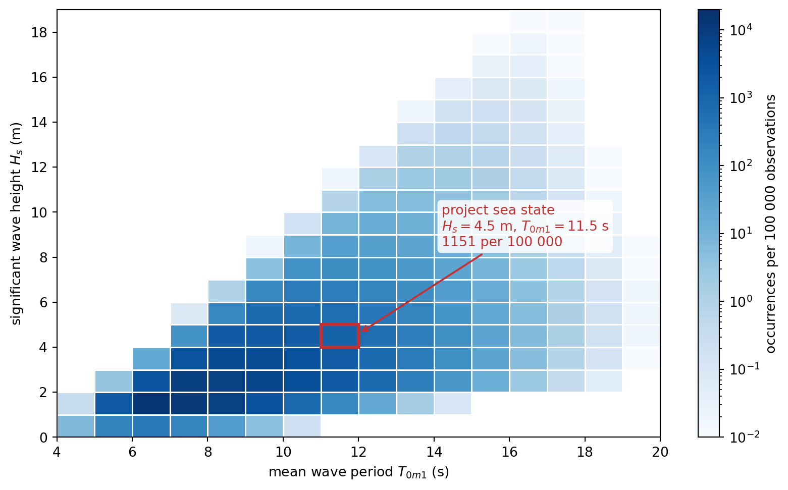
The scatter diagram in numbers, and why it matters
| \(H_s\) \ \(T_{0m1}\) | 4.5 | 5.5 | 6.5 | 7.5 | 8.5 | 9.5 | 10.5 | 11.5 | 12.5 | 13.5 | 14.5 | 15.5 | 16.5 | 17.5 | 18.5 | 19.5 | Sum |
|---|---|---|---|---|---|---|---|---|---|---|---|---|---|---|---|---|---|
| 0.5 | 6.82 | 202.00 | 333.61 | 187.76 | 45.59 | 4.74 | 0.21 | 780.73 | |||||||||
| 1.5 | 0.33 | 2028.35 | 12750.82 | 11693.39 | 7215.76 | 3006.80 | 846.07 | 160.77 | 20.63 | 1.79 | 0.10 | 37724.81 | |||||
| 2.5 | 3.38 | 2805.81 | 8517.74 | 7835.85 | 5885.37 | 3608.30 | 1805.81 | 737.71 | 246.00 | 66.96 | 14.88 | 2.70 | 0.40 | 0.05 | 31530.96 | ||
| 3.5 | 23.06 | 2742.51 | 4666.81 | 4100.83 | 2936.41 | 1713.38 | 814.68 | 315.65 | 99.66 | 25.64 | 5.38 | 0.92 | 0.13 | 0.01 | 17445.07 | ||
| 4.5 | 82.06 | 1759.81 | 2069.19 | 1715.42 | 1151.29 | 625.51 | 275.12 | 97.96 | 28.24 | 6.59 | 1.24 | 0.19 | 0.02 | 7812.64 | |||
| 5.5 | 0.08 | 149.74 | 811.81 | 791.81 | 609.66 | 375.67 | 185.26 | 73.12 | 23.09 | 5.84 | 1.18 | 0.19 | 0.02 | 3027.47 | |||
| 6.5 | 1.02 | 147.59 | 305.37 | 271.71 | 190.23 | 104.79 | 45.42 | 15.49 | 4.16 | 0.88 | 0.15 | 0.02 | 1086.83 | ||||
| 7.5 | 4.77 | 88.62 | 107.20 | 86.26 | 53.35 | 25.36 | 9.27 | 2.60 | 0.56 | 0.09 | 0.01 | 378.09 | |||||
| 8.5 | 0.02 | 9.40 | 38.70 | 36.80 | 25.95 | 13.63 | 5.33 | 1.55 | 0.34 | 0.05 | 0.01 | 131.78 | |||||
| 9.5 | 0.20 | 9.34 | 15.15 | 12.51 | 7.39 | 3.12 | 0.94 | 0.20 | 0.03 | 48.88 | |||||||
| 10.5 | 0.81 | 5.73 | 5.96 | 4.08 | 1.90 | 0.60 | 0.13 | 0.02 | 19.23 | ||||||||
| 11.5 | 0.02 | 1.29 | 2.68 | 2.23 | 1.18 | 0.40 | 0.08 | 0.01 | 7.89 | ||||||||
| 12.5 | 0.11 | 1.01 | 1.14 | 0.72 | 0.27 | 0.06 | 0.01 | 3.32 | |||||||||
| 13.5 | 0.22 | 0.51 | 0.42 | 0.18 | 0.04 | 1.37 | |||||||||||
| 14.5 | 0.02 | 0.19 | 0.21 | 0.12 | 0.03 | 0.57 | |||||||||||
| 15.5 | 0.04 | 0.09 | 0.07 | 0.02 | 0.22 | ||||||||||||
| 16.5 | 0.03 | 0.04 | 0.01 | 0.08 | |||||||||||||
| 17.5 | 0.01 | 0.02 | 0.01 | 0.04 | |||||||||||||
| 18.5 | 0.01 | 0.01 | 0.02 | ||||||||||||||
| Sum | 7.15 | 2233.73 | 15913.30 | 23223.54 | 21674.58 | 16031.12 | 10301.81 | 5868.69 | 2909.77 | 1230.31 | 437.79 | 129.62 | 31.47 | 6.11 | 0.92 | 0.09 | 100000 |
Dividing a cell by \(100\,000\) gives the probability that the sea is in that state at a random moment, or the fraction of its time at sea that a ship spends in it. The row and column sums give the probabilities of \(H_s\) and of \(T_{0m1}\) alone.
This project is a short-term analysis: the response of the ship to one sea state. A long-term analysis repeats it for every cell and weights each result by the probability of its cell. That is how the fatigue damage of a hull is accumulated, or how the operability of a ship is found: the fraction of the time for which a criterion, such as an upper limit on the MSI, is met.
11.4.1 The spectrum
IACS Recommendation 34 prescribes a JONSWAP spectrum with peak enhancement factor \(\gamma = 1.5\):
\[\begin{align} S_{\eta\eta}(\omega) = \alpha\, \frac{5}{16} H_s^2\, \omega_p^4\, \omega^{-5} \exp\left[-\frac{5}{4}\left(\frac{\omega_p}{\omega}\right)^4\right] \gamma^{\exp\left[-\frac{(\omega/\omega_p - 1)^2}{2\sigma^2}\right]} \end{align}\]
with \(\omega_p = 2\pi/T_p\), \(\sigma = 0.07\) for \(\omega \le \omega_p\) and \(0.09\) above, and the normalizing factor
\[\begin{align} \alpha = \frac{1}{5}\left(\frac{1}{0.1160 + 0.0594\sqrt{\gamma} + 0.0246\,\gamma}\right) \end{align}\]
The period of the scatter diagram is not the peak period
The period of the IACS scatter diagram is defined from the spectral moments \(m_n = \int_0^\infty \omega^n S_{\eta\eta}\,d\omega\) as \(T_{0m1} = 2\pi m_{-1}/m_0\), the energy period. It is neither \(T_p\) nor the mean period \(2\pi m_0/m_1\). For this spectrum
\[\begin{align} T_{0m1} = \left(0.7757 + 0.0965\sqrt{\gamma} - 0.0144\,\gamma\right) T_p \end{align}\]
so \(T_{0m1} = 11.5\) s means \(T_p = 13.18\) s.
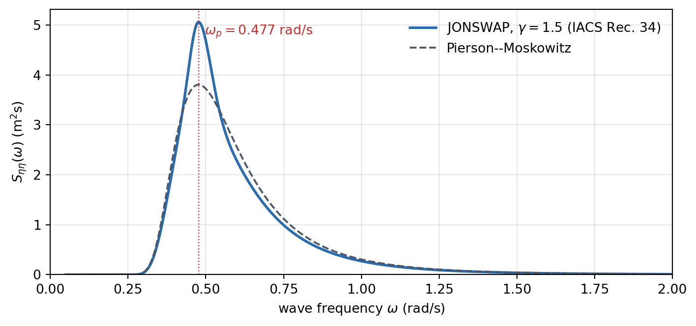
Check your spectrum against Table 11.6 and Figure 11.2 before going further. The sea is long-crested: all the wave energy travels in the single direction \(\beta\).
| Quantity | Value |
|---|---|
| Peak period \(T_p\) | \(13.18\) s |
| Peak frequency \(\omega_p\) | \(0.4766\) rad/s |
| Normalizing factor \(\alpha\) | \(0.8863\) |
| Peak spectral density \(S_{\eta\eta}(\omega_p)\) | \(5.06\) m\(^2\)s |
| \(m_0\) (check: \(H_s^2/16 = 1.2656\) m\(^2\)) | \(1.2653\) m\(^2\) |
| \(2\pi m_{-1}/m_0\) (check: \(T_{0m1}\)) | \(11.50\) s |
11.5 Step 2: The Motions of the Ship
The panel method HydRA has solved the radiation and diffraction problems for every hull, heading, speed and wave frequency. In the download of each hull (Table 11.3), the file matlab/<member>_hydra.json (or the equivalent .mat file) holds everything you need, in SI units (Table 11.7). The frequencies run from \(0.1\) to \(1.5\) rad/s in steps of \(0.1\) rad/s, after an entry for infinite frequency (a negative value) and one for \(\omega = 0\) whose values are all zero: drop both.
| Key | Shape | Content |
|---|---|---|
w |
\([n_\omega]\) | wave frequencies \(\omega\), rad/s |
beta |
\([n_\beta]\) | headings \(\beta\), in radians (\(\pi\) is head seas) |
speed |
\([n_U]\) | speeds \(U\), m/s |
M, C |
\([6, 6]\) | rigid-body mass and hydrostatic restoring matrices about \(O\) |
AM, BD |
\([n_\omega, 6, 6, n_\beta, n_U]\) | added mass \(\boldsymbol{A}\) and radiation damping \(\boldsymbol{B}\) |
Fk_Re, Fk_Im, Fs_Re, Fs_Im |
\([n_\omega, 6, n_\beta, n_U]\) | Froude–Krylov and scattering loads per metre of wave amplitude |
rao_Re, rao_Im |
\([n_\omega, 6, n_\beta, n_U]\) | HydRA’s RAOs, without viscous damping; rotations in rad/m |
Conventions
- BCS: \(x\) to the bow, \(y\) to port, \(z\) up, origin \(O\) at midship on the centreline in the calm waterline. Positive pitch is bow down.
- \(\beta\) is the direction in which the waves travel, measured from \(+x\): \(180^\circ\) is head seas, and in beam and bow quartering seas the waves come from starboard.
- Complex amplitudes multiply \(e^{i\omega_e t}\); phases are relative to the wave crest at \(O\) (Chapter 8).
- Use the speeds of the results file and \(g = 9.80665\) m/s\(^2\), the value used by HydRA. The water is deep.
The RAOs follow from the equations of motion of Chapter 8, solved at every frequency, heading and speed:
\[\begin{align} \left[-\omega_e^2\left(\boldsymbol{M} + \boldsymbol{A}(\omega_e)\right) + i\omega_e\left(\boldsymbol{B}(\omega_e) + \boldsymbol{B}_v\right) + \boldsymbol{C}\right]\{\hat{\xi}\} = \{\hat{F}_{FK} + \hat{F}_{S}\} \end{align}\]
A panel method finds only the damping due to the waves that the hull radiates. That is enough for heave and pitch, but for roll it is tiny: the real roll damping comes from viscous effects at the bilges and bilge keels. Add a linear viscous roll damping of \(5\%\) of critical, the only non-zero element of \(\boldsymbol{B}_v\):
\[\begin{align} B_{v,44} = 0.05 \times 2\sqrt{C_{44}\left(M_{44} + A_{44}(\omega_n)\right)}, \qquad \omega_n = \sqrt{\frac{C_{44}}{M_{44} + A_{44}(\omega_n)}} \end{align}\]
Find the roll natural frequency \(\omega_n\) by iteration, with \(A_{44}\) in beam seas at the design speed, and use the same \(B_{v,44}\) for every heading and speed of a hull.
Before you trust your RAOs
- Check your code. With \(\boldsymbol{B}_v = 0\), your solution must reproduce HydRA’s RAOs at the computed frequencies to round-off accuracy.
- Resolve the resonances. The roll resonance peak is only a few hundredths of a rad/s wide, far narrower than the \(0.1\) rad/s spacing of the data. Interpolate \(\boldsymbol{A}\), \(\boldsymbol{B}\) and \(\{\hat{F}\}\) (the loads through their real and imaginary parts), which vary smoothly, onto a fine grid, and solve the equations of motion there. Do not interpolate the RAOs.
- Look out for irregular frequencies. At certain frequencies, above roughly \(\omega_{irr}^2 = gk\coth(kT)\) with \(k = \pi\sqrt{1/L_{pp}^2 + 1/B^2}\) (an encounter frequency), a panel method of this kind produces narrow, spurious spikes. Plot the coefficients against \(\omega_e\) for the five speeds together: a point where one speed departs abruptly from its neighbours is a spike. Replace it, and report which points you replaced.
- Taper the RAOs in short waves. In head and bow quartering seas, bring the RAOs smoothly to zero, for example with a cosine taper, over the last \(10\%\) below the wave frequency at which the wavelength is a quarter of the ship length, \(\lambda = L_{pp}/4\), that is \(\omega = \sqrt{8\pi g/L_{pp}}\). Waves this short hardly move the hull along its length, but the acceleration weights them by \(\omega_e^4\), so any spurious values of the panel method there add energy that is not real. In beam seas a wave runs across the beam, not the length, and still moves the ship at these frequencies: do not taper there. Check that the taper changes your MSI only slightly.
11.6 Step 3: The Vertical Acceleration of the Cabin
From the RAOs, derive the spectrum \(S_{aa}(\omega_e)\) of the vertical acceleration of the cabin, and its moments
\[\begin{align} m_n^a = \int_0^\infty \omega_e^n\, S_{aa}(\omega_e)\, d\omega_e, \qquad \sigma_a = \sqrt{m_0^a}, \qquad \bar{\omega}_e = \frac{m_1^a}{m_0^a} \end{align}\]
This derivation is the heart of the project. Everything you need is in Chapter 7 (the encounter frequency), Chapter 8 (the complex RAO and the vertical motion of a point of the hull) and Section 9.15 (the response spectrum, its moments, and the encounter spectrum at forward speed). Show your derivation in the report and state every assumption.
11.7 Step 4: The Motion Sickness Incidence
In motion simulator experiments with about a thousand young men, O’Hanlon, McCauley and co-workers (O’Hanlon and McCauley 1974; McCauley et al. 1976) found that the percentage who vomit within two hours of vertical oscillation grows with the logarithm of the acceleration as a cumulative normal distribution, and that people are most susceptible at about \(0.16\) Hz. Their fit (O’Hanlon and McCauley 1974; Journée and Pinkster 2002) is
\[\begin{align} \text{MSI} = 100\, \Phi\left(\frac{\log_{10}(\bar{a}/g) - \mu_{MSI}}{0.4}\right) \ [\%], \qquad \mu_{MSI} = -0.819 + 2.32\left(\log_{10}\bar{\omega}_e\right)^2 \end{align}\]
where \(\bar{a}\) is the mean value of the absolute vertical acceleration in m/s\(^2\), \(\bar{\omega}_e\) its frequency in rad/s, and \(\Phi\) the cumulative distribution function of the standard normal distribution. The frequency dependence is built into \(\mu_{MSI}\), so the acceleration needs no frequency weighting. Figure 11.3 shows the model: at the most sensitive frequency, \(1\) rad/s, a mean acceleration of \(1.49\) m/s\(^2\) makes half the people sick.

The model was fitted to sinusoidal motion. For the random acceleration of a ship we use two definitions, so that all groups can be compared:
- Magnitude: the acceleration is a zero-mean Gaussian process, so the mean of its absolute value is \(\bar{a} = \sqrt{2/\pi}\,\sigma_a \approx 0.798\,\sigma_a\).
- Frequency: \(\bar{\omega}_e = m_1^a/m_0^a\), the mean frequency of the acceleration spectrum.
The error function is not \(\Phi\)
Some texts write the model with an “erf” defined as \(\frac{1}{\sqrt{2\pi}}\int_0^z e^{-t^2/2}\,dt\), which is \(\Phi(z) - 0.5\). The standard error function of NumPy, SciPy and MATLAB is different: use \(\Phi(z) = \frac{1}{2}\left[1 + \text{erf}(z/\sqrt{2})\right]\), or scipy.stats.norm.cdf(z).
| \(\bar{a}\) (m/s\(^2\)) | \(\bar{\omega}_e\) (rad/s) | MSI (%) |
|---|---|---|
| \(0.5\) | \(0.6\) | \(7.1\) |
| \(0.8\) | \(1.2\) | \(23.9\) |
| \(1.0\) | \(1.0\) | \(33.3\) |
| \(2.0\) | \(0.8\) | \(60.5\) |
11.8 Deliverables
Each group submits a report, with the code that produced every number in it. The report should contain:
- The derivation of the acceleration spectrum of the cabin, with all assumptions stated.
- The roll damping and the data: \(\omega_n\) and \(B_{v,44}\) of both hulls, their wave-making roll damping at \(\omega_n\) as a fraction of critical, and the computed points you replaced as spikes.
- A results table for both hulls and all \(15\) combinations of heading and speed: \(U\), \(\sigma_a\), \(\bar{a}\), \(\bar{\omega}_e\), \(\mu_{MSI}\) and the MSI.
- Plots of
- the roll RAO of both hulls in beam seas at \(Fn_{des}\), with and without the viscous roll damping
- the MSI against \(Fn/Fn_{des}\), one curve per heading, baseline and variant on the same axes
- the acceleration spectra of both hulls at \(Fn_{des}\), for each heading
- all \(30\) cases on the \((\bar{\omega}_e, \bar{a})\) plane over contours of constant MSI
- A discussion, one parameter at a time:
- The hull. Which hull is more comfortable, at which headings and speeds, and by how much? Explain it through the RAOs.
- Speed. How does the MSI change with speed in each heading? Is the change driven by \(\bar{a}\) or by \(\bar{\omega}_e\)?
- Heading. Which heading is worst for your hulls? Which modes contribute to the acceleration in each heading?
- The cabin. Repeat one head-sea case with the cabin at midship (\(x_P = 0\)), and one beam-sea case with the cabin on the centreline (\(y_P = 0\)) and on the starboard side (\(y_P = -0.4B\)). Where would you put the cabin?
- Roll damping. Repeat one beam-sea case with \(\zeta_v = 0.025\) and \(0.10\). Explain the result from where \(\omega_n\) lies relative to the wave spectrum.
- Limitations. The population of the experiments, the two hour exposure, a model for sinusoidal motion applied to random motion, the long-crested sea, the linear RAOs and the assumed roll damping: which would make your MSI an overestimate, and which an underestimate?
Before you trust your numbers, ask whether each is physically sensible. What should \(\sigma_a\) do as the speed increases in head seas? Which modes can contribute in head seas, and which in beam seas? Does the result change when you halve the frequency step? A worked solution will be released after the project.
11.9 Summary
- The project chains four steps: the equations of motion with a viscous roll damping, the vertical acceleration of the cabin, its spectrum in the design sea state, and the MSI.
- The sea state is the IACS Rec. 34 JONSWAP spectrum with \(H_s = 4.5\) m and \(T_{0m1} = 11.5\) s; the period of the scatter diagram is the energy period, so \(T_p = 13.18\) s.
- The O’Hanlon and McCauley model gives the MSI from the mean absolute acceleration \(\bar{a} = \sqrt{2/\pi}\,\sigma_a\) and the mean frequency \(\bar{\omega}_e = m_1^a/m_0^a\); people are most susceptible near \(1\) rad/s.
- The discussion looks at one parameter at a time: the hull, the speed, the heading, the position of the cabin and the roll damping.