9 Irregular Waves in the Ocean

Learning Objectives

After reading this chapter, you should be able to:

Describe the wave elevation at a point as a stochastic process, and explain the terms random variable, realization and ensemble.
Define the PDF and CDF of a random variable and the joint PDF and CDF of a stochastic process.
Distinguish stationarity from ergodicity, and explain why ergodicity lets a single wave record stand in for the whole ensemble.
State the properties of a stationary Gaussian process, and compute its mean, moments and variance.
Relate the autocorrelation function to the joint PDF of $\eta_t$ and $\eta_{t+\tau}$, and estimate it from a measured record.
Relate the autocorrelation function to the power spectral density through the Wiener–Khintchine relations, and convert between one-sided and two-sided spectra, between $\omega$ and $f$, and between their spectral moments.
Use Rice’s results to compute the expected rates of upcrossings and peaks, the bandwidth $\varepsilon$ and the distribution of peaks, including $H_s = 4\sqrt{m_0}$ and the means of the highest $1/n$ of the peaks.
Write down the Pierson–Moskowitz and JONSWAP spectra in terms of $H_s$, $T_p$ and $\gamma$, and describe a directional wave spectrum.
Compute the response spectrum of a linear system from the input spectrum and the system’s transfer function.
Compute the response spectrum of a floating structure from the wave spectrum and its RAOs, and estimate the statistics of the response: its significant amplitude, the rate at which it exceeds a level, and its largest value in a sea state.

9.1 Motivation

The content up to the previous chapter has described the calculation of the response of a ship or offshore platform to an irregular ocean wave by expressing it as a sum of regular waves through the idea of Fourier transform. The response to each regular wave is computed and added together to get the response of the floating structure to the irregular wave. While an ocean wave time history is irregular, it does have defined statistical properties. This chapter discusses the statistics of wave elevation in the ocean and also about the statistics of a response of a structure subjected to such a sea.

9.2 Random Variable

The outcomes of a random experiment can numerically be represented by a random variable. For example, consider the experiment of rolling a die. We can represent the outcome of the experiment (the number that faces up when the die is rolled) as the random variable $X$. In this example the random variable $X$ can only take on discrete values from $1$ to $6$. Now consider the current stock price of a company. This too is random and can be represented by a random variable, say $Y$. However, the stock price is continuous and can take on any value between $[0,\infty)$. In a similar manner, we can consider the current wave elevation at a specific location (say 500 m off the coast of Marina Beach, Chennai) to be a continuous random variable $\eta$ that can take on values between $(-\infty, \infty)$.

9.3 Stochastic (or Random) Process

Now we know that the wave elevation at a specific location does change with time. If we measure the wave elevation at this particular location (say 500 m off the coast of Marina Beach, Chennai) using a wave probe, we observe one wave realization of the underlying stochastic process $\left\{\eta_t\right\}$, where $t \in [t_i, t_f]$ and $t_i$ and $t_f$ denote an initial and a final time respectively. Note that $\left\{\eta_t\right\}$ is a stochastic process, where the wave elevation at each continuous time $t$ is represented by a random variable $\eta_t$. A combination of infinitely many such random variables $\eta_t$ corresponding to $t \in [t_i, t_f]$ when put together results in the stochastic process $\left\{\eta_t\right\}$. A stochastic process is also known as a random process.

9.4 Probability Density Function and Cumulative Distribution Function

For simplicity, let’s consider a discrete set of times $t_i = t_1, t_2, ..., t_n$ and the stochastic process $\left\{\eta_{t} \right\}$. Each of $\eta_{t_i}$ is a random variable and is characterized by a cumulative distribution function (CDF) $P_{\eta_{t_i}}(\eta_0)$:

\[\begin{align} P_{\eta_{t_i}}(\eta_0) = \operatorname{Prob}[\eta_{t_i} \leq \eta_0] \end{align}\]

$P_{\eta_{t_i}}(\eta_0)$ denotes the probability that the value of the random variable $\eta_{t_i}$ is less than or equal to a threshold $\eta_0$. Note that $0 \leq P_{\eta_{t_i}}(\eta_0) \leq 1$ and $P_{\eta_{t_i}}(-\infty) = 0$ and $P_{\eta_{t_i}}(\infty) = 1$. The probability density function $p_{\eta_{t_i}}(\eta_0)$ is defined as:

\[\begin{align} p_{\eta_{t_i}}(\eta_0) = \frac{dP}{d\eta_0} (\eta_0) \end{align}\]

and $p_{\eta_{t_i}}(\eta_0) \Delta \eta_0$ denotes the probability that $\eta_{t_i}$ lies between $\eta_0$ and $\eta_0 + \Delta \eta_0$ in the limit $\Delta \eta_0 \rightarrow 0$. Similar to a random variable, the joint CDF of the process $\left\{\eta_t\right\}$ is denoted by $P_{\eta}(\eta_{1}, \eta_{2}, ..., \eta_{n})$ and is defined as:

\[\begin{align} P_{\eta}(\eta_{1}, \eta_{2}, ..., \eta_{n}) = \operatorname{Prob}\left[\eta_{t_1} \leq \eta_1, \eta_{t_2} \leq \eta_2, ..., \eta_{t_n} \leq \eta_n\right] \end{align}\]

where $t_i = t_1, t_2, ..., t_n$ and $t_i \in (-\infty, \infty)$. The joint probability density function of stochastic process $\left\{\eta_t\right\}$ is denoted by $p_{\eta}(\eta_{1}, \eta_{2}, ..., \eta_{n})$. Note that the joint PDF $p_{\eta}(\eta_{1}, \eta_{2}, ..., \eta_{n})$ denotes the following probability:

\[\begin{align} p_{\eta}(\eta_{1}, \eta_{2}, ..., \eta_{n}) = \lim_{\Delta \eta_i \rightarrow 0} \frac{\operatorname{Prob}\left[\eta_1 \leq \eta_{t_1} \leq \eta_1 + \Delta \eta_1, ..., \eta_n \leq \eta_{t_n} \leq \eta_n + \Delta \eta_n\right]}{\Delta \eta_1 \Delta \eta_2 ... \Delta \eta_n} \end{align}\]

9.5 Concept of Ensemble

When a die is rolled once, you may observe the value $5$. This is known as a realization of the random variable $X$. While this instance turned up the number $5$, it could have (equally likely) turned up any other number between $1$ and $6$. The set of all possible realizations is termed as an ensemble. Similarly, for a random process $\left\{\eta_{t} \right\}$ when we collect data using a wave probe at a specific location, we have sampled one wave time history realization from the ensemble (consisting of infinitely many possible realizations).

9.6 Stationarity and Ergodicity

A random process $\left\{\eta_{t} \right\}$ is said to be stationary if its joint CDFs are unchanged by a shift of the time origin, that is, if for every $n$, every set of times $t_1, ..., t_n$ and every time shift $T$:

\[\begin{align} \operatorname{Prob}\left[\eta_{t_1} \leq \eta_1, ..., \eta_{t_n} \leq \eta_n\right] = \operatorname{Prob}\left[\eta_{t_1+T} \leq \eta_1, ..., \eta_{t_n+T} \leq \eta_n\right] \end{align}\]

A stochastic process $\left\{\eta_{t} \right\}$ is said to be ergodic if it is stationary and all temporal averages taken along a single realization are equal to corresponding expectations formed by taking averages across the ensemble. The ensemble average for the wave elevation at a specific location and time (denoted by the random variable $\eta_t$) is given by:

\[\begin{align} E[\eta_t] = \lim_{N\rightarrow\infty} \frac{1}{N} \sum_{i=1}^{N} \eta_t^{(i)} \end{align}\]

where $\eta_t^{(i)}$ denotes the $i^{th}$ realization from the ensemble of the random variable $\eta_t$. Ergodicity implies that:

\[\begin{align} E[\eta_t] &= \lim_{T \rightarrow \infty} \frac{1}{T} \int_{t_1}^{t_1 + T} \eta^{(i)}(\tau) d\tau \\ E[\eta_t^2] &= \lim_{T \rightarrow \infty} \frac{1}{T} \int_{t_1}^{t_1 + T} \left(\eta^{(i)}(\tau)\right)^2 d\tau \end{align}\]

for an arbitrary $t_1$ and an arbitrary $i$. Note that the $\eta^{(i)}(\tau)$ is the $i^{th}$ realization of the stochastic process from the ensemble. If a stochastic process is ergodic, then the measured realization $\eta^{(i)}(\tau)$ is typical of all other possible realizations such that the variation of the wave elevation with respect to time may be used to represent the different possible realizations of wave elevation $\eta_t$ at one particular time $t$. Mathematically, this enables us to replace the expected value (averaged over ensemble) by the temporal average. Notice that an ergodic process must be stationary but a stationary process need not be ergodic.

9.6.1 Stationary but NOT Ergodic

Consider the example of a random process that is either always $+1$ or always $-1$, chosen randomly at the beginning. This process is defined as:

\[\begin{align} X(t) = A \qquad \forall t \end{align}\]

with:

\[\begin{align} P(A=+1) = P(A=-1) = \frac{1}{2} \end{align}\]

The CDF at time $t$ is invariant with time. Similarly, the joint probabilities of the process at two times $t_1$ and $t_2$ do not change with time:

\[\begin{align} P(X_{t_1} = +1, X_{t_2} = +1) = \frac{1}{2} \\ P(X_{t_1} = -1, X_{t_2} = +1) = 0 \\ P(X_{t_1} = +1, X_{t_2} = -1) = 0 \\ P(X_{t_1} = -1, X_{t_2} = -1) = \frac{1}{2} \\ \end{align}\]

This can be extended for joint CDF across multiple times too. As the CDF and joint CDFs are all invariant with time, this process is strictly stationary. The ensemble average for the process at any time $t$ is given by:

\[\begin{align} E[X_t] = E[A] = 0 \end{align}\]

However, the temporal average across any one realization is defined as:

\[\begin{align} <X> = \lim_{T \rightarrow \infty} \frac{1}{T} \int_{-T/2}^{T/2} X^{(i)}(\tau) d\tau \end{align}\]

Now $<X>$ is either $+1$ or $-1$ depending on which realization $X^{(i)}$ is chosen. As the temporal average of the process does not equal the ensemble average, the process, even though being stationary, is not ergodic.

9.6.2 Wind Generated Waves in the Ocean

The waves in the ocean are formed by the wind blowing over the surface of the ocean for long periods of time and over long distances (the distance over which the wind blows is known as the fetch). Due to wind shear, ripples are formed on the water surface. This undulated surface allows wind to transfer more energy to form larger waves on the water surface. The different wave components interact with each other and after sufficient time has passed, the waves reach a statistical stationarity. Such a sea is called a fully developed sea and the wave elevation in such seas can be assumed to be stationary and ergodic. However, there are limits to this stationarity and ergodicity assumptions. As the wind changes (as it does when a storm comes by), the statistical properties of the sea also undergo a change. In general as a rule of thumb, one can assume that the sea waves have a stationary and ergodic behaviour over a period of 2-3 hours. Thus in this sense the waves can be thought of as being short-term stationary (or quasi-stationary).

9.7 Identically Distributed Process

For a generic stochastic process $\left\{\eta_{t} \right\}$, each random variable $\eta_{t}$ can have its own PDF different from the PDF of the process at a different time. However, for a stationary process the joint PDF and joint CDF do not change under a time shift, and this makes the process identically distributed. Thus the PDF of process at any time can be represented by the same PDF $p_{\eta}(\eta_0) \equiv p_{\eta_t}(\eta_0)$. Notice that this does not mean that the random variables corresponding to two different times are independent. We will explicitly cover this when we discuss autocorrelation functions below.

9.8 Gaussian Process

A stochastic process $\left\{\eta_t\right\}$ is called a Gaussian process if each random variable $\eta_t$ follows a Gaussian distribution and the random variables $(\eta_{t_1}, \eta_{t_2}, ..., \eta_{t_n})$ for any $n$ also follow a multivariate Gaussian distribution. The PDF of the random variable $\eta_t$ is given by the PDF of the Gaussian distribution:

\[\begin{align} p_{\eta_t}(x) = \frac{1}{\sigma_{\eta_t}\sqrt{2\pi}} \exp\left(- \frac{(x - \mu_{\eta_t})^2}{2\sigma_{\eta_t}^2}\right) \end{align}\]

where $\mu_{\eta_t} = E[\eta_t]$ is the mean value of $\eta_t$ and $\sigma_{\eta_t}$ is the standard deviation of $\eta_t$. The CDF of $\eta_t$ is given by:

\[\begin{align} P_{\eta_t}(x) = \Phi\left(\frac{x-\mu_{\eta_t}}{\sigma_{\eta_t}}\right) = \frac{1}{2}\left(1 + \operatorname{erf}\left(\frac{x-\mu_{\eta_t}}{\sigma_{\eta_t}\sqrt{2}}\right)\right) \end{align}\]

where $\Phi(.)$ is the CDF of the standard normal distribution (with zero mean and unit variance) and the error function $\operatorname{erf}(.)$ is defined as:

\[\begin{align} \operatorname{erf}(x) = \frac{2}{\sqrt{\pi}} \int_{0}^{x} e^{-t^2}dt \end{align}\]

The Gaussian PDF and CDF are characterized by two parameters $\mu_{\eta_t}$ and $\sigma_{\eta_t}$. If the process is stationary, then each $\eta_t$ for all values of $t$ will have the same PDF and CDF given by:

\[\begin{align} p_{\eta}(x) &= \frac{1}{\sigma_{\eta}\sqrt{2\pi}} \exp\left(- \frac{(x - \mu_{\eta})^2}{2\sigma_{\eta}^2}\right) \\ P_{\eta}(x) &= \Phi\left(\frac{x-\mu_{\eta}}{\sigma_{\eta}}\right) = \frac{1}{2}\left(1 + \operatorname{erf}\left(\frac{x-\mu_{\eta}}{\sigma_{\eta}\sqrt{2}}\right)\right) \end{align}\]

Interactive Gaussian PDF and CDF

The mean $\mu_{\eta}$ is the elevation at which the PDF peaks, and the elevation at which the CDF equals one half. The standard deviation $\sigma_{\eta}$ sets the width: a smaller $\sigma_{\eta}$ produces a taller, narrower PDF and a steeper CDF. Use the sliders below to change $\mu_{\eta}$, $\sigma_{\eta}$ and a threshold elevation $x$. The shaded area under the PDF to the left of $x$ is $P_{\eta}(x)$, read off the CDF at the same elevation. The dashed curve is the standard normal distribution ($\mu = 0$, $\sigma = 1$), drawn on the same axes. The marker can also be dragged across either plot.

Mean, $\mu$ (m): 0.00

Standard deviation, $\sigma$ (m): 1.00

Threshold, $x$ (m): 0.00

Reference curve Standard normal, $\mu = 0$, $\sigma = 1$

Wave elevation in metres. About 68.3% of the probability lies within one standard deviation of the mean, and about 95.4% within two. Those fractions do not depend on $\mu$ or $\sigma$.

Probability density function $p(x)$

Cumulative distribution function $P(x)$

$p(x)$ m⁻¹

$P(x) = \mathrm{Prob}(\eta \le x)$

peak density $1/(\sigma\sqrt{2\pi})$ m⁻¹

$\mathrm{Prob}(\eta \le \mu)$0.500

9.9 Common Statistical Measures

Some of the commonly used statistical measures are defined below.

Mean

\[\begin{align} \mu_{\eta} = E[\eta] = \int_{-\infty}^{\infty} x p_{\eta}(x) dx \end{align}\]

For a Gaussian random variable $\eta$ characterized by $\mu$ and $\sigma$, the mean value is given by:

\[\begin{align} E[\eta] = \int_{-\infty}^{\infty} x \frac{1}{\sigma\sqrt{2\pi}} \exp\left(- \frac{(x - \mu)^2}{2\sigma^2}\right) dx = \mu \end{align}\]

Expected value of any function $g(\eta)$

\[\begin{align} E[g(\eta)] = \int_{-\infty}^{\infty} g(x) p_{\eta}(x) dx \end{align}\]

$n^{th}$ moment

\[\begin{align} E[(\eta)^n] = \int_{-\infty}^{\infty} x^n p_{\eta}(x) dx \label{eq-nth-moment} \end{align}\]

Mean square value

The mean square value is the second moment of the random variable and is given by:

\[\begin{align} E[(\eta)^2] = \int_{-\infty}^{\infty} x^2 p_{\eta}(x) dx \end{align}\]

Central $n^{th}$ moment

\[\begin{align} E\left[\left(\eta - E[\eta]\right)^n\right] = \int_{-\infty}^{\infty} \left(x - E[\eta]\right)^n p_{\eta}(x) dx \end{align}\]

For a Gaussian random variable $\eta$ characterized by $\mu$ and $\sigma$, $n^{th}$ central moments are given by:

\[\begin{align} E[(\eta - E[\eta])^n] = E[(\eta - \mu)^n] = \begin{cases} 0 & \text{if $n$ is odd} \\ & \\ \sigma^n (n-1)!! & \text{if $n$ is even} \end{cases} \end{align}\]

where

\[\begin{align} (n-1)!! = \prod_{k=1}^{n/2} (2k - 1) = 1 \cdot 3 \cdot 5 \cdots (n-1) \qquad \text{for even $n$} \end{align}\]

Variance

\[\begin{align} \sigma_{\eta}^2 = E\left[\left(\eta - E[\eta]\right)^2\right] = \int_{-\infty}^{\infty} \left(x - E[\eta]\right)^2 p_{\eta}(x) dx \end{align}\]

If the random variable $\eta$ has zero mean, $\mu_{\eta} = E[\eta] = 0$, then the standard deviation is equal to the root mean square value:

\[\begin{align} \sigma_{\eta} = \sqrt{E\left[\left(\eta\right)^2\right]} \end{align}\]

For a Gaussian random variable characterized by $\mu$ and $\sigma$, the variance is given by $\sigma_{\eta}^2 = \sigma^2$.

9.10 Autocorrelation function

The autocorrelation function is defined as:

\[\begin{align} R_{\eta\eta}(\tau) = E\left[\eta_{t}\eta_{t+\tau}\right] =\int_{-\infty}^{\infty} \int_{-\infty}^{\infty} x y ~p_{\eta_t \eta_{t+\tau}} (x, y) dx ~dy \end{align}\]

where $p_{\eta_t \eta_{t+\tau}} (x, y)$ is the joint PDF of $\eta_t$ and $\eta_{t+\tau}$. The autocorrelation function is the expected value of the product of the two random variables $\eta_{t}$ and $\eta_{t+\tau}$. A large positive value of autocorrelation means that the random variables $\eta_{t}$ and $\eta_{t+\tau}$ are strongly correlated. If $R_{\eta\eta}(\tau)$ is large and positive, it means that positive values of $\eta_{t}$ are likely observed together with positive values of $\eta_{t+\tau}$. If $R_{\eta\eta}(\tau)$ is large and negative, it means that positive values of $\eta_{t}$ are likely observed together with negative values of $\eta_{t+\tau}$. $R_{\eta\eta}(\tau) = 0$ implies that $\eta_{t}$ and $\eta_{t+\tau}$ are uncorrelated: there is no linear trend connecting them. For a Gaussian process uncorrelated random variables are also independent, but this is not true in general.

The autocorrelation at zero lag is the mean square value $R_{\eta\eta}(0) = E\left[\eta_t^2\right]$. The magnitude of the autocorrelation function at any non-zero lag is bounded by its value at zero lag.

\[\begin{align} |R_{\eta\eta}(\tau)| \leq R_{\eta\eta}(0) \end{align}\]

The autocorrelation function is an even function of the lag time $\tau$.

\[\begin{align} R_{\eta\eta}(-\tau) = R_{\eta\eta}(\tau) \end{align}\]

For a zero mean process, the autocorrelation coefficient is defined as shown below and is bounded $-1 \leq \rho_{\eta\eta}(\tau) \leq 1$. For a process with a non-zero mean, the autocovariance $R_{\eta\eta}(\tau) - \mu_{\eta}^2$ replaces the autocorrelation in both the numerator and the denominator.

\[\begin{align} \rho_{\eta\eta} (\tau) = \frac{R_{\eta\eta}(\tau)}{R_{\eta\eta}(0)} \end{align}\]

If a stochastic process is ergodic, the ensemble mean can be replaced by the temporal mean and the autocorrelation can be expressed as:

\[\begin{align} R_{\eta\eta}(\tau) &= E\left[\eta_{t}\eta_{t+\tau}\right] = <\eta^{(i)}(t) \eta^{(i)}(t+\tau)> \nonumber\\ &= \lim_{T\rightarrow\infty} \frac{1}{T} \int_{-T/2}^{T/2} \eta^{(i)}(t) \eta^{(i)}(t+\tau) dt \end{align}\]

where $\eta^{(i)}(t)$ for $t \in [-T/2, T/2]$ is a finite time realization (some arbitrary $i^{th}$ realization of the ensemble of infinitely many possible realizations) of the stochastic process $\left\{\eta_t\right\}$.

If the stochastic process $\left\{\eta_t\right\}$ is a stationary Gaussian process, then the joint PDF of $\eta_{t}$ and $\eta_{t+\tau}$ is a multivariate normal distribution whose PDF is given by:

\[\begin{align} p_{\eta_t \eta_{t+\tau}} (x, y) = \frac{1}{2\pi \sqrt{\det(\boldsymbol{\Sigma}_{\tau})}} \exp \left(-\frac{1}{2} \left(\begin{Bmatrix}x \\ y\end{Bmatrix} - \begin{Bmatrix}\mu_1 \\ \mu_2\end{Bmatrix}\right)^T \boldsymbol{\Sigma}_{\tau}^{-1} \left(\begin{Bmatrix}x \\ y\end{Bmatrix} - \begin{Bmatrix}\mu_1 \\ \mu_2\end{Bmatrix}\right)\right) \end{align}\]

where $\mu_1 = E[\eta_t]$ and $\mu_2 = E[\eta_{t+\tau}]$ and the covariance matrix $\boldsymbol{\Sigma}_{\tau}$ is given by:

\[\begin{align} \boldsymbol{\Sigma}_{\tau} = \begin{bmatrix} E[(\eta_{t} - \mu_1)^2] & E[(\eta_{t} - \mu_1)(\eta_{t+\tau} - \mu_2)] \\ E[(\eta_{t+\tau} - \mu_2)(\eta_{t} - \mu_1)] & E[(\eta_{t+\tau} - \mu_2)^2] \end{bmatrix} \end{align}\]

If the process is zero mean, then the covariance matrix $\boldsymbol{\Sigma}_{\tau}$ is given by:

\[\begin{align} \boldsymbol{\Sigma}_{\tau} = \begin{bmatrix} E[\eta_{t}^2] & E[\eta_{t}\eta_{t+\tau}] \\ E[\eta_{t+\tau}\eta_{t}] & E[\eta_{t+\tau}^2] \end{bmatrix} = \begin{bmatrix} R_{\eta\eta}(0) & R_{\eta\eta}(\tau) \\ R_{\eta\eta}(\tau) & R_{\eta\eta}(0) \end{bmatrix} \end{align}\]

It can be seen that the covariance matrix $\boldsymbol{\Sigma}_{\tau}$ is always symmetric and positive semi-definite. The value of $R_{\eta\eta}(\tau)$ influences the joint PDF and determines how observed samples of $\eta_t$ and $\eta_{t+\tau}$ will be correlated.

Key point

Note that in general for a non-Gaussian random process, the joint PDF cannot be uniquely determined from its autocorrelation function. However, for a zero-mean Gaussian process, the autocorrelation function uniquely determines the joint PDF of the process.

Interactive Wave Record, Histogram and Joint PDF

The explorer below connects a single measured wave record to the probability densities defined above. The record is one realization of a sea described by the Pierson–Moskowitz spectrum in its $H_s$, $T_p$ form (see Section 9.13)

\[\begin{align} S_{\eta\eta}(\omega) = \frac{5}{16} H_s^2 \omega_p^4 \omega^{-5} \exp\left(-\frac{5}{4}\left(\frac{\omega_p}{\omega}\right)^4\right), \qquad \omega_p = \frac{2\pi}{T_p} \end{align}\]

synthesized as a sum of many cosine components $\eta(t) = \sum_n \sqrt{2 S_{\eta\eta}(\omega_n)\Delta\omega} \cos(\omega_n t + \varphi_n)$ with independent, uniformly distributed random phases $\varphi_n$. The record is sampled at $\Delta t = 0.25$ s, giving $N$ values $\eta_i = \eta(i\Delta t)$.

Because the process is ergodic, each sample $\eta_i$ of this one record can stand in for a draw of $\eta_t$ from the ensemble. Collecting all the samples of the record onto the vertical axis gives the histogram drawn to the right of the time history. It approaches the Gaussian PDF with zero mean and variance $R_{\eta\eta}(0) = m_0 \approx H_s^2/16$.

The same idea extends to two times. For a lag $\tau = k\Delta t$, every time $t_i$ in the record gives one pair $(\eta_i, \eta_{i+k})$, which is a draw of $(\eta_t, \eta_{t+\tau})$ from the joint PDF $p_{\eta_t\eta_{t+\tau}}(x, y)$. The highlighted pair in the time history is the orange dot in the joint histogram. Binning all $N - k$ pairs gives the 2D histogram, and averaging their products gives the ergodic estimate of the autocorrelation:

\[\begin{align} \hat{R}_{\eta\eta}(\tau) = \frac{1}{N-k} \sum_{i=1}^{N-k} \eta_i \, \eta_{i+k} \end{align}\]

This is the discrete form of the temporal average above. The dashed ellipses are contours of the bivariate normal density with covariance matrix $\boldsymbol{\Sigma}_{\tau}$ built from $R_{\eta\eta}(0)$ and $R_{\eta\eta}(\tau)$ of the spectrum, through the Wiener–Khintchine relation. Their principal axes lie along $y = \pm x$, with variances $R_{\eta\eta}(0) \pm R_{\eta\eta}(\tau)$, so the sign and size of $R_{\eta\eta}(\tau)$ set which way the cloud of pairs leans and how thin it is. The dotted line $y = \rho_{\eta\eta}(\tau)\, x$ is the expected value of $\eta_{t+\tau}$ given $\eta_t = x$.

Things to try:

Press Play to measure the record from the start. Each new sample drops into the histogram on the right, and each new pair $(\eta(t-\tau), \eta(t))$ lands in the joint histogram. The histograms start ragged and fill out towards the Gaussian shapes, while $\hat{R}_{\eta\eta}(\tau)$ settles onto $R_{\eta\eta}(\tau)$. The time averages approach the ensemble averages as the record grows.
Set $\tau = 0$. Every pair is $(\eta, \eta)$, the cloud collapses onto the diagonal, and $\hat{R}_{\eta\eta}(0)$ is the mean square value of the record.
Increase $\tau$ to about $0.4\,T_p$. A crest at $t$ is now usually followed by a trough at $t + \tau$, so $\rho_{\eta\eta}(\tau) \approx -0.65$ and the cloud leans the other way. Near $\tau \approx 0.9\,T_p$ the correlation is positive again ($\rho_{\eta\eta} \approx 0.3$), and at long lags the cloud becomes nearly circular.
Shorten the record to 2 minutes and press New realization a few times. The histograms become ragged and $\hat{R}_{\eta\eta}(\tau)$ wanders around $R_{\eta\eta}(\tau)$. With a 3 hour record the time averages settle close to the ensemble values, which is what ergodicity promises in the limit $T \rightarrow \infty$.
Change $H_s$. Every elevation scales with $H_s$, so the shapes stay fixed and only the axis values change. Changing $T_p$ stretches the autocorrelation function along the lag axis.

Significant wave height, $H_s$ (m): 4.00

Peak period, $T_p$ (s): 10.0

Lag, $\tau$ (s): 1.00

Record length, $T$: 20 min

Playback speed: 10×

Play measures the record from $t = 0$ up to the playhead. The histograms and time averages include only the samples measured so far, and the orange dots mark the newest pair $(\eta(t-\tau), \eta(t))$. Drag along the time history, or the strip below it, to move the playhead. Drag across the autocorrelation plot to change $\tau$, even while the record plays.

Wave elevation record $\eta(t)$ and the histogram of its samples

Joint histogram of $(\eta(t), \eta(t+\tau))$ and the joint normal PDF

Autocorrelation function $R_{\eta\eta}(\tau)$

samples / pairs measured so far

temporal mean $\langle \eta \rangle$ m

$\hat{R}(0)$ record / $R(0)$ spectrum m²

$\hat{R}(\tau)$ record / $R(\tau)$ spectrum m²

$\hat{\rho}(\tau)$ record / $\rho(\tau)$ spectrum

9.11 Power Spectral Density

The two-sided power spectral density $S_{\eta\eta}^{(2)}(\omega)$ is defined as the Fourier transform of the autocorrelation function $R_{\eta\eta}(\tau)$. Note that a two-sided power spectral density is defined for the range $\omega \in (-\infty, \infty)$.

\[\begin{align} S_{\eta\eta}^{(2)}(\omega) = \int_{-\infty}^{\infty} R_{\eta\eta}(\tau) e^{-i\omega \tau} d\tau \label{eq-psd-autocorr} \end{align}\]

Similarly, the inverse transform of the two-sided power spectral density yields the autocorrelation function.

\[\begin{align} R_{\eta\eta}(\tau) = \frac{1}{2\pi}\int_{-\infty}^{\infty} S_{\eta\eta}^{(2)}(\omega) e^{i\omega \tau} d\omega \label{eq-autocorr-psd} \end{align}\]

The pair of equations $\eqref{eq-psd-autocorr}$ and $\eqref{eq-autocorr-psd}$ are known as the Wiener-Khintchine relations.

Consider a finite duration (or truncated) realization $\eta_T(t)$ of the random process $\left\{\eta_t\right\}$ for $t \in [-T/2, T/2]$. Assuming that the process is ergodic, the autocorrelation function of this finite duration realization $R_{\eta\eta}^T(\tau)$ can be represented as:

\[\begin{align} R_{\eta\eta}^T(\tau) = \frac{1}{T} \int_{-\infty}^{\infty} \eta_T(t)\eta_T(t+\tau) dt \label{eq-autocorrelation-truncated} \end{align}\]

Note that while the integral is defined from $-\infty$ to $\infty$, $R_{\eta\eta}^T(\tau)$ only assumes non-zero values for the lag values where the two finite duration signals overlap. In the limit $T \rightarrow \infty$, the autocorrelation function of the finite duration realization $R_{\eta\eta}^T(\tau)$ will approach $R_{\eta\eta}(\tau)$.

\[\begin{align} \lim_{T\rightarrow \infty} R_{\eta\eta}^T(\tau) = R_{\eta\eta}(\tau) \end{align}\]

The corresponding power spectral density for the finite duration realization $S_{\eta\eta}^{(2)T}(\omega)$ is given by:

\[\begin{align} S_{\eta\eta}^{(2)T}(\omega) = \int_{-\infty}^{\infty} R_{\eta\eta}^T(\tau) e^{-i\omega \tau} d\tau \end{align}\]

Substituting $\eqref{eq-autocorrelation-truncated}$ leads to:

\[\begin{align} S_{\eta\eta}^{(2)T}(\omega) &= \int_{-\infty}^{\infty} \frac{1}{T} \int_{-\infty}^{\infty} \eta_T(t)\eta_T(t+\tau) dt ~ e^{-i\omega \tau} d\tau \nonumber \\ &= \frac{1}{T} \int_{-\infty}^{\infty} \int_{-\infty}^{\infty} \eta_T(t)\eta_T(t+\tau) e^{-i\omega \tau} d\tau ~dt \end{align}\]

Substituting a change of variable $u=t+\tau$ yields:

\[\begin{align} S_{\eta\eta}^{(2)T}(\omega) &= \frac{1}{T} \int_{-\infty}^{\infty} \int_{-\infty}^{\infty} \eta_T(t)\eta_T(u) e^{-i\omega (u-t)} du ~dt \nonumber \\ &= \frac{1}{T} \int_{-\infty}^{\infty} \eta_T(t) \int_{-\infty}^{\infty} \eta_T(u) e^{-i\omega u} du~ e^{i\omega t}~dt \nonumber \\ &= \frac{1}{T} \int_{-\infty}^{\infty} \eta_T(t) \hat{\eta}_T(\omega) ~ e^{i\omega t}~dt \nonumber \\ &= \frac{1}{T} \hat{\eta}_T^{*}(\omega) \hat{\eta}_T(\omega) = \frac{|\hat{\eta}_T(\omega)|^2}{T} \end{align}\]

where $(.)^{*}$ is the complex conjugate operator. As the observation duration increases $(T \rightarrow \infty)$, the estimated autocorrelation $R_{\eta\eta}^T(\tau)$ approaches the true autocorrelation $R_{\eta\eta}(\tau)$ at every lag under the ergodicity assumption. The quantity $|\hat{\eta}_T(\omega)|^2/T$, known as the periodogram, does not settle down in the same way. Computed from a single record it scatters about the true spectrum, and its scatter does not shrink as $T$ grows: a longer record resolves more frequencies instead of averaging each frequency more. The limit holds for the expected value of the periodogram over the ensemble:

\[\begin{align} S_{\eta\eta}^{(2)}(\omega) = \lim_{T\rightarrow \infty} E\left[S_{\eta\eta}^{(2)T}(\omega)\right] = \lim_{T\rightarrow \infty} \frac{E\left[|\hat{\eta}_T(\omega)|^2\right]}{T} \end{align}\]

In practice the expectation is approximated by averaging. A long record is split into shorter segments and their periodograms are averaged, or the periodogram is smoothed over neighbouring frequencies. Both trade frequency resolution for a steadier estimate.

Since $R_{\eta\eta}(\tau)$ is real and even, $S_{\eta\eta}^{(2)}(\omega)$ is also real and even. Setting $\tau = 0$ in $\eqref{eq-autocorr-psd}$ gives

\[\begin{align} R_{\eta\eta}(0) = \frac{1}{2\pi}\int_{-\infty}^{\infty} S_{\eta\eta}^{(2)}(\omega) d\omega = \frac{1}{\pi}\int_{0}^{\infty} S_{\eta\eta}^{(2)}(\omega) d\omega \end{align}\]

The one-sided spectrum is defined for $\omega \geq 0$ such that its integral over positive frequencies equals the mean square value $R_{\eta\eta}(0)$. It is related to the two-sided spectrum as:

\[\begin{align} S_{\eta\eta}(\omega) = \frac{1}{2\pi}\left[S_{\eta\eta}^{(2)}(\omega) + S_{\eta\eta}^{(2)}(-\omega)\right] = \frac{1}{\pi} S_{\eta\eta}^{(2)}(\omega) \qquad \omega \geq 0 \end{align}\]

In practice we work with the one-sided spectrum of the circular frequency $\omega$ or cyclic frequency $f = \omega/2\pi$, where

\[\begin{align} S_{\eta\eta}(f) = S_{\eta\eta}(\omega) \frac{d\omega}{df} = 2\pi S_{\eta\eta}(\omega) \end{align}\]

The spectrum is an important feature of a random process and denotes how the energy in the process is distributed across different frequencies. Just as we computed the $n^{th}$ moments of a random variable in $\eqref{eq-nth-moment}$, we can compute the moments of the spectrum too. These moments characterize the distribution of the spectral energy in the random process across frequencies.

\[\begin{align} m_n = \int_{0}^{\infty} \omega^n S_{\eta\eta}(\omega) d\omega \label{eq-spectral-moments} \end{align}\]

Throughout this book spectral moments are taken with respect to the circular frequency $\omega$, as in $\eqref{eq-spectral-moments}$. The zeroth order spectral moment is the mean square value and for a zero mean process reduces to the variance.

\[\begin{align} m_0 &= \int_{0}^{\infty} S_{\eta\eta}(\omega) d\omega = \int_{0}^{\infty} S_{\eta\eta}(f) df \nonumber\\ &= R_{\eta\eta}(0) = E[\eta_t^2] = \sigma_{\eta}^2 \end{align}\]

Much of the literature uses moments with respect to the cyclic frequency $f$ instead. We write these as $m_n^{(f)}$. Since $S_{\eta\eta}(f) df = S_{\eta\eta}(\omega) d\omega$ and $\omega = 2\pi f$, they are related by:

\[\begin{align} m_n^{(f)} = \int_{0}^{\infty} f^n S_{\eta\eta}(f) df = \frac{m_n}{(2\pi)^n} \end{align}\]

The two agree for $n = 0$, and dimensionless ratios of moments such as the bandwidth $\varepsilon$ below are the same in both. Rates and periods differ by factors of $2\pi$, so when using a formula from another source, check which convention it uses.

9.12 Distribution of Upcrossings and Peaks

While the joint PDF describes the variation of the random process, it does not bring out certain statistical properties such as:

The statistical distribution of zero-crossing of the process
The statistical distribution of the peaks of the process

Rice (1944, 1945) showed that for a stationary zero mean Gaussian random process $\left\{\eta_t\right\}$, the expected number of upcrossings per unit time past a given threshold $\eta_0$ is given by:

\[\begin{align} E[N_{+}(\eta_0)] = \frac{1}{2\pi}\sqrt{\frac{m_2}{m_0}} \exp\left( - \frac{\eta_0^2}{2m_0}\right) \end{align}\]

where $m_2$ and $m_0$ are the second and zeroth moments $\eqref{eq-spectral-moments}$ of the one-sided spectrum $S_{\eta\eta}(\omega)$. The factor $1/2\pi$ turns the circular frequency $\sqrt{m_2/m_0}$ into a number of crossings per unit time; with cyclic moments the same result reads $E[N_{+}(\eta_0)] = \sqrt{m_2^{(f)}/m_0^{(f)}} \exp(-\eta_0^2/2m_0)$. Defining a peak or a local maximum as random variable $A$ where $\dot{\eta}(t) = 0$ and $\ddot{\eta}(t) < 0$, the probability of $A$ occurring between $a$ and $a + \Delta a$ in the limit $\Delta a \rightarrow 0$ is the PDF of A and is defined as:

\[\begin{align} \operatorname{Prob}[a < A \leq a + \Delta a] = p_{A}(a) \Delta a \end{align}\]

Rice (1944, 1945) further showed that the probability density function of the peaks of a stationary zero mean Gaussian process is given by:

\[\begin{align} p_{A}(a) &= \frac{\varepsilon}{\sqrt{2\pi m_0}} \exp \left(-\frac{a^2}{2 m_0 \varepsilon^2}\right) \nonumber \\ & + \sqrt{1 - \varepsilon^2} \frac{a}{m_0} \exp\left(-\frac{a^2}{2 m_0}\right) \left[\frac{1}{2} + \frac{1}{2}\operatorname{erf}\left\{\frac{a}{\sqrt{m_0}} \frac{\sqrt{1-\varepsilon^2}}{\varepsilon\sqrt{2}}\right\}\right] \end{align}\]

where $0 \leq \varepsilon \leq 1$ is the bandwidth and defined as:

\[\begin{align} \varepsilon^2 = 1 - \frac{m_2^2}{m_0m_4} \end{align}\]

For a narrow banded process $\varepsilon \rightarrow 0$,

\[\begin{align} p_{A}(a) &= \frac{a}{m_0} \exp\left(-\frac{a^2}{2 m_0}\right) & 0 \leq a \leq \infty \end{align}\]

This is the Rayleigh distribution. Integrating it from $0$ to $a$ gives the CDF of the peaks:

\[\begin{align} P_{A}(a) = 1 - \exp\left(-\frac{a^2}{2 m_0}\right) = 1 - \exp\left(-\frac{a^2}{2 \sigma_{\eta}^2}\right) \label{eq-rayleigh-cdf} \end{align}\]

A single parameter, the variance of the process $m_0 = \sigma_{\eta}^2$, fixes the whole distribution. Here $\sigma_{\eta}$ plays the role of the scale parameter of the Rayleigh distribution. It is not the standard deviation of the peaks $A$, which works out to $\sqrt{(2 - \pi/2) m_0} \approx 0.655\sqrt{m_0}$. Inverting $\eqref{eq-rayleigh-cdf}$ gives the peak level associated with a given non-exceedance probability:

\[\begin{align} \frac{a^2}{m_0} = -2 \ln\left(1 - P_{A}(a)\right) = -4.605 \log_{10}\left(1 - P_{A}(a)\right) \end{align}\]

As an example, setting $P_{A}(a) = 0.99$ shows that roughly one peak in every hundred rises above $3.03 \sqrt{m_0}$.

At the other extreme, a broad banded process ($\varepsilon \rightarrow 1$) has peaks that follow the same Gaussian distribution as the process itself, and the peaks can therefore be negative:

\[\begin{align} p_{A}(a) &= \frac{1}{\sqrt{2\pi m_0}} \exp\left(-\frac{a^2}{2 m_0}\right) & -\infty < a < \infty \end{align}\]

Rice (1944, 1945) also showed that the expected number of peaks per unit time is

\[\begin{align} E[N_{p}] = \frac{1}{2\pi}\sqrt{\frac{m_4}{m_2}} \end{align}\]

Whatever the bandwidth, dividing the zero upcrossing rate $E[N_{+}(0)] = \frac{1}{2\pi}\sqrt{m_2/m_0}$ by the peak rate links the two counts to $\varepsilon$:

\[\begin{align} \frac{E[\text{no. of zero upcrossings per unit time}]}{E[\text{no. of peaks per unit time}]} = \frac{\sqrt{m_2/m_0}}{\sqrt{m_4/m_2}} = \frac{m_2}{\sqrt{m_0 m_4}} = \sqrt{1 - \varepsilon^2} \end{align}\]

As $\varepsilon \rightarrow 0$ the ratio tends to one, so a narrow banded process has, on average, exactly one peak between successive zero upcrossings.

9.12.1 Narrow Band Gaussian Processes

Because a narrow band process has one peak per upcrossing, every zero upcrossing almost certainly starts a new complete oscillation. The rate of zero upcrossings $E[N_{+}(0)]$ is then the expected cyclic frequency $f_0 = \omega_0/2\pi$ of the process, where

\[\begin{align} \omega_0^2 = \frac{m_2}{m_0} = \frac{\int_{0}^{\infty} \omega^2 S_{\eta\eta}(\omega) d\omega}{\int_{0}^{\infty} S_{\eta\eta}(\omega) d\omega} \end{align}\]

and the mean zero upcrossing period, also written $T_z$, is its reciprocal:

\[\begin{align} \bar{T}_0 = \frac{1}{f_0} = \frac{2\pi}{\omega_0} = 2\pi\sqrt{\frac{m_0}{m_2}} \end{align}\]

A time history of a narrow band process looks like a sinusoid at frequency $\omega_0$ whose amplitude and phase drift slowly and randomly, and its spectrum is a sharp spike centred on $\omega_0$. In the limit, the spectrum can be idealized as a Dirac delta function carrying the total variance $S_0$:

\[\begin{align} S_{\eta\eta}(\omega) &= S_0 \delta(\omega - \omega_0) & \text{where} \quad \int_{0}^{\infty} S_{\eta\eta}(\omega) d\omega = S_0 \end{align}\]

Its spectral moments follow directly from the sifting property of the delta function:

\[\begin{align} m_0 &= S_0 \nonumber \\ m_2 &= \omega_0^2 S_0 \nonumber \\ m_4 &= \omega_0^4 S_0 \end{align}\]

and substituting them into the bandwidth confirms that the idealized process is perfectly narrow banded:

\[\begin{align} \varepsilon^2 = 1 - \frac{m_2^2}{m_0 m_4} = 1 - \frac{(\omega_0^2 S_0)^2}{S_0 (\omega_0^4 S_0)} = 0 \end{align}\]

Statistics of the Highest Peaks

Design quantities are often based on the largest peaks rather than on a typical peak. Define $a_{1/n}$ as the level that only the highest $1/n$ fraction of the peaks exceed. Using the Rayleigh distribution,

\[\begin{align} \operatorname{Prob}[A > a_{1/n}] &= 1 - P_{A}(a_{1/n}) \nonumber\\ &= \int_{a_{1/n}}^{\infty} p_{A}(a) da \nonumber\\ &= \int_{a_{1/n}}^{\infty} \frac{a}{m_0} \exp\left(-\frac{a^2}{2 m_0}\right) da \nonumber\\ &= \exp\left(-\frac{a_{1/n}^2}{2 m_0}\right) = \frac{1}{n} \end{align}\]

and solving for the threshold gives $a_{1/n}^2 = 2 m_0 \ln(n)$.

The mean of the peaks lying above this threshold, denoted $<a_{1/n}>$, is the first moment of the tail of the distribution divided by the probability $1/n$ contained in that tail:

\[\begin{align} <a_{1/n}> &= \frac{1}{1/n} \int_{a_{1/n}}^{\infty} a\, p_{A}(a) da = n \int_{a_{1/n}}^{\infty} \frac{a^2}{m_0} \exp\left(-\frac{a^2}{2 m_0}\right) da \nonumber \\ &= n\sqrt{2 m_0} \left[\frac{1}{n}\sqrt{\ln(n)} + \frac{\sqrt{\pi}}{2}\left(1 - \operatorname{erf}\left\{\sqrt{\ln(n)}\right\}\right)\right] \label{eq-avg-1-n-highest} \end{align}\]

Evaluating $\eqref{eq-avg-1-n-highest}$ for a few values of $n$ gives the standard results. With $n = 1$ the tail is the whole distribution, so the result is the mean peak amplitude:

\[\begin{align} <a> = \int_{0}^{\infty} a\, p_{A}(a) da = 1.25\sqrt{m_0} \end{align}\]

With $n = 3$ the result is the mean of the highest third of the peaks, called the significant amplitude:

\[\begin{align} <a_{1/3}> = 2.0\sqrt{m_0} \end{align}\]

With $n = 10$ the result is the mean of the highest tenth of the peaks:

\[\begin{align} <a_{1/10}> = 2.55\sqrt{m_0} \end{align}\]

In a narrow band Gaussian process each crest is followed by a trough of the same size, so a peak-to-peak (crest to trough) height is twice the amplitude. The significant height is therefore

\[\begin{align} H_S = <H_{1/3}> = 2<a_{1/3}> = 4.0\sqrt{m_0} \end{align}\]

and the mean of the highest tenth of the peak-to-peak heights is

\[\begin{align} <H_{1/10}> = 2<a_{1/10}> \approx 5.1\sqrt{m_0} \end{align}\]

9.12.2 Wide Band Processes

In a wide band process the time history oscillates rapidly about a slowly varying level, so several local maxima occur between successive zero crossings and some of them lie below the mean. Three idealized wide band spectra are commonly used:

Ideal white noise, with $S_{\eta\eta}(\omega) = S_0$ constant for all $0 < \omega < \infty$. This is a mathematical convenience only: the area under the spectrum, and hence the mean square value of the process, is infinite, so no physical process can be white. Results derived with this idealization should be used with care.
Band-limited white noise, with $S_{\eta\eta}(\omega) = S_0$ for $\omega_1 < \omega < \omega_2$ and zero elsewhere.
White noise with a cut-off frequency, with $S_{\eta\eta}(\omega) = S_0$ for $0 < \omega < \omega_c$ and zero elsewhere.

Interactive Upcrossings and Peaks

The explorer below counts the upcrossings and peaks of a synthesized wave record and compares them with Rice’s results computed from the spectrum. The Pierson–Moskowitz and JONSWAP spectra of Section 9.13 cannot be used here, because their $m_4$, and hence $\varepsilon$, depends on where the spectrum is cut off. To sweep the bandwidth with a single slider, the spectrum is instead built from two Gaussian peaks in $f$, for which every moment is finite. A narrow primary peak sits at $f_p = 0.1$ Hz ($T_p = 10$ s). A small secondary peak at $5 f_p$ stands for short waves riding on the longer ones. The slider sets $\varepsilon$, and the share of the variance placed in the secondary peak is adjusted until the spectral moments give that $\varepsilon$. The spectrum is scaled so that $m_0 = 1$ m², which makes an elevation in metres the same number as the elevation in units of $\sqrt{m_0}$. The values in the table can therefore be compared directly with the results above, such as $<a> = 1.25\sqrt{m_0}$ and $<a_{1/3}> = 2.0\sqrt{m_0}$.

The record is sampled at $\Delta t = T_p/128$. A peak is a local maximum of the samples, refined by fitting a parabola through the three samples around it. An upcrossing of a level $\eta_0$ is a step from a sample below $\eta_0$ to a sample at or above it. As in the previous explorer, Play measures the record from $t = 0$ up to the playhead. Each new peak drops into the vertical histogram of peaks, next to the Rice PDF. The upcrossing rate of every level is drawn against $E[N_{+}(\eta_0)]$ in the panel on the far right.

Notice how little energy it takes to make a process wide banded. At $\varepsilon = 0.9$ the secondary peak holds only about 1.3% of the variance, yet the number of peaks per unit time is more than 2.5 times that of the narrow band case. This happens because $m_4$ weights each frequency by $\omega^4$, so a small amount of high-frequency energy dominates it. The spectrum is drawn on a log scale so that the small secondary peak stays visible. The zero upcrossing rate, which depends on $m_2$, changes far less, and $H_{1/3}$ of the zero upcrossing waves stays close to $4\sqrt{m_0}$.

Things to try:

Set $\varepsilon$ to its smallest value, about 0.13, and press Play. Almost every wave has a single crest, so there is about one peak per zero upcrossing. The peak histogram builds up into the Rayleigh shape.
Increase $\varepsilon$ to 0.5 and then 0.9. The short waves add peaks between the zero crossings, and some of these peaks lie below the mean (hollow markers). The histogram spreads into negative values and moves towards the Gaussian limit. The fraction of negative peaks approaches $(1 - \sqrt{1-\varepsilon^2})/2$.
Raise the threshold to $\eta_0 = 3$ m. Upcrossings become rare, so the counts from a 10 minute record scatter widely about the expected number, while a 3 hour record settles close to it.
Compare the columns of the table. As $\varepsilon$ grows, $<a>$, $<a_{1/3}>$ and $<a_{1/10}>$ of the record fall below the narrow band (Rayleigh) values and follow the Rice values instead.

Bandwidth, $\varepsilon$: 0.40

Threshold, $\eta_0$ (m): 2.0

Record length, $T$: 1 h

Playback speed: 50×

Play measures the record from $t = 0$ up to the playhead. The histogram, the upcrossing rates and the table include only the part measured so far. Drag along the time history, or the strip below it, to move the playhead. The spectrum has $m_0 = 1$ m², so $\sqrt{m_0} = 1$ m and $H_s = 4$ m.

record so far peak negative peak upcrossing of $\eta_0$ peak histogram Rice, from the spectrum Rayleigh ($\varepsilon = 0$) and Gaussian ($\varepsilon = 1$) limits upcrossing rate of the record

Record $\eta(t)$ with its peaks and upcrossings, the peak histogram $p_A(a)$, and the upcrossing rate $E[N_+(\eta)]$ of every level

Spectrum $S_{\eta\eta}(f)$ on a log scale, with the zero upcrossing rate $E[N_+(0)] = \frac{1}{2\pi}\sqrt{m_2/m_0}$ and the peak rate $E[N_p] = \frac{1}{2\pi}\sqrt{m_4/m_2}$

Statistic	Record	Rice, from spectrum	Narrow band, $\varepsilon \to 0$

9.13 Wave Spectra

9.13.1 Models for One-Dimensional Frequency Spectra

In this book a short-term sea state is specified by two numbers: the significant wave height $H_s = 4\sqrt{m_0}$ and the peak period $T_p$, the period at which the spectrum has its maximum ($\omega_p = 2\pi/T_p$, $f_p = 1/T_p$). The two standard spectra below are written in this form, following DNV-RP-C205 (Det Norske Veritas 2010). Wave scatter diagrams often give a mean period instead, such as the energy period $T_{0m1}$ of the IACS diagram used in the project; it must first be converted to $T_p$ for the chosen spectrum.

Pierson–Moskowitz spectrum

\[\begin{align} S_{\eta\eta}(\omega) = \frac{5}{16} H_s^2\, \omega_p^4\, \omega^{-5} \exp\left[-\frac{5}{4}\left(\frac{\omega}{\omega_p}\right)^{-4}\right] \label{eq-pierson-moskowitz} \end{align}\]

or, in terms of cyclic frequency using $S_{\eta\eta}(f) = 2\pi S_{\eta\eta}(\omega)$,

\[\begin{align} S_{\eta\eta}(f) = \frac{5}{16} H_s^2\, f_p^4\, f^{-5} \exp\left[-\frac{5}{4}\left(\frac{f}{f_p}\right)^{-4}\right] \label{eq-pierson-moskowitz-f} \end{align}\]

The substitution $u = \frac{5}{4}\omega_p^4 \omega^{-4}$ gives $\int_0^\infty \omega^{-5} \exp\left(-\frac{5}{4}\omega_p^4\omega^{-4}\right) d\omega = 1/(5\omega_p^4)$, so that

\[\begin{align} m_0 = \int_0^\infty S_{\eta\eta}(\omega)\, d\omega = \frac{H_s^2}{16} \end{align}\]

and $H_s = 4\sqrt{m_0}$ holds exactly. The mean zero upcrossing period of this spectrum is $T_z = 2\pi\sqrt{m_0/m_2} \approx T_p/1.41$. The same two-parameter form appears under several names in the literature: the Bretschneider (Bretschneider 1959) or ISSC spectrum, the modified (or two-parameter) Pierson–Moskowitz spectrum, and, in offshore practice, simply the Pierson–Moskowitz spectrum.

When the wind has blown for long enough over a long enough fetch, the waves stop growing and the sea is said to be fully developed. Its significant wave height and peak period are then tied together, approximately as

\[\begin{align} T_p \approx 5.0\sqrt{H_s} \qquad (T_p \text{ in seconds}, H_s \text{ in metres}) \end{align}\]

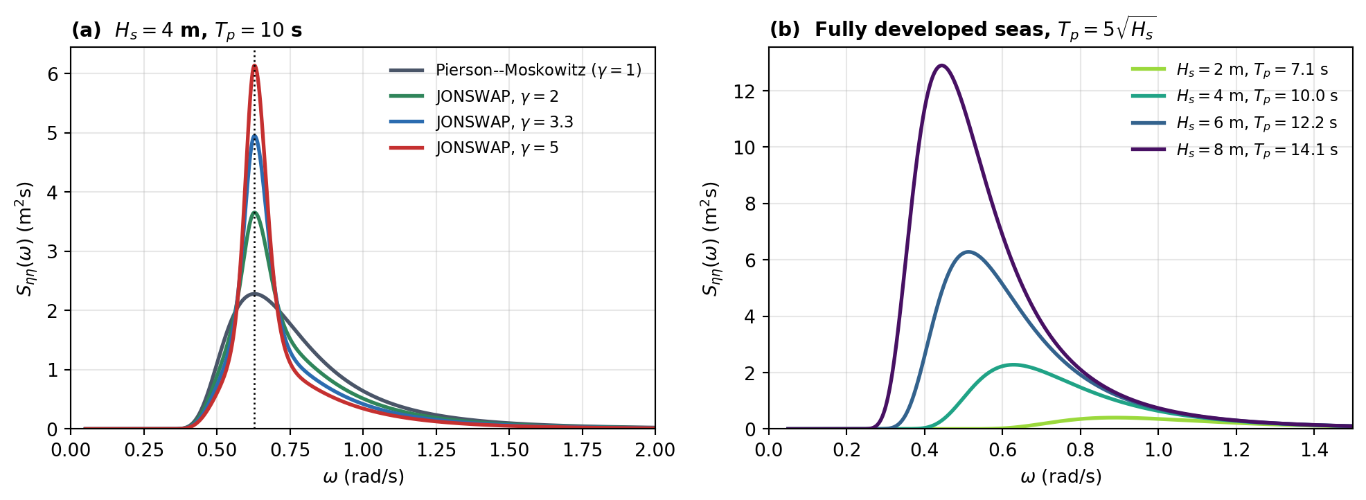
so that, for example, a fully developed sea with $H_s = 4$ m has $T_p \approx 10$ s (Figure 9.1(b)). The two-parameter form $\eqref{eq-pierson-moskowitz}$ lets $H_s$ and $T_p$ be chosen independently. A younger, steeper sea that is still growing has a shorter peak period than $5\sqrt{H_s}$, and is better described by the JONSWAP spectrum.

Background: the original Pierson–Moskowitz spectrum in terms of wind speed

This is included for reference only; you do not need to remember these formulas. In this course every sea state is given by $H_s$ and $T_p$.

Pierson and Moskowitz (Pierson and Moskowitz 1964) originally proposed a one-parameter spectrum for a fully developed sea, specified by the mean wind speed $U_{19.5}$ measured 19.5 m above the sea surface:

\[\begin{align} S_{\eta\eta}(\omega) = \alpha g^2 \omega^{-5} \exp\left[-\beta\left(\frac{g}{U_{19.5}\,\omega}\right)^4\right], \qquad \alpha = 0.0081, \quad \beta = 0.74 \label{eq-pierson-moskowitz-wind} \end{align}\]

Setting $dS_{\eta\eta}/d\omega = 0$ places its peak at $\omega_p = (4\beta/5)^{1/4} g/U_{19.5} = 0.877\, g/U_{19.5}$, and comparing with $\eqref{eq-pierson-moskowitz}$ shows that it is the special case $\alpha g^2 = \frac{5}{16} H_s^2 \omega_p^4$. This is where the fully developed relation above comes from:

\[\begin{align} H_s \approx 0.21 \frac{U_{19.5}^2}{g}, \qquad \omega_p \approx 0.40\sqrt{\frac{g}{H_s}}, \qquad T_p \approx 5.0\sqrt{H_s} \end{align}\]

For example, a wind of $U_{19.5} = 13.7$ m/s produces a fully developed sea with $H_s = 4$ m and $T_p = 10$ s.

JONSWAP spectrum

The Joint North Sea Wave Project (Hasselmann et al. 1973) measured seas that were still growing under a steady offshore wind, limited by the fetch. Their spectra have the same $\omega^{-5}$ high-frequency tail as the Pierson–Moskowitz spectrum, but a sharper and higher peak. In terms of $H_s$ and $T_p$ the JONSWAP spectrum is written as a modification of $\eqref{eq-pierson-moskowitz}$ (Det Norske Veritas 2010):

\[\begin{align} S_{\eta\eta}(\omega) = A_\gamma\, S_{PM}(\omega)\, \gamma^{\exp\left[-\frac{(\omega - \omega_p)^2}{2\sigma^2\omega_p^2}\right]} \label{eq-jonswap} \end{align}\]

where $S_{PM}(\omega)$ is the Pierson–Moskowitz spectrum $\eqref{eq-pierson-moskowitz}$ with the same $H_s$ and $T_p$, and

\[\begin{align} \sigma = \begin{cases} 0.07 & \text{for } \omega \leq \omega_p \\ 0.09 & \text{for } \omega > \omega_p \end{cases} \qquad\qquad A_\gamma = 1 - 0.287 \ln\gamma \end{align}\]

The exponent of $\gamma$ equals one at $\omega = \omega_p$ and falls to zero within a few multiples of $\sigma\omega_p$ on either side, so the peak enhancement factor $\gamma$ raises the spectrum near the peak and leaves the rest of it unchanged. Raising the peak would also raise the area under the spectrum, so the normalizing factor $A_\gamma$ brings $m_0$ back to $H_s^2/16$. It is an approximation: the resulting $m_0$ differs from $H_s^2/16$ by less than 2% for $1 \leq \gamma \leq 7$. With $\gamma = 1$, $A_\gamma = 1$ and $\eqref{eq-jonswap}$ reduces to the Pierson–Moskowitz spectrum. The average of the JONSWAP measurements is $\gamma = 3.3$.

Figure 9.1(a) compares the two spectra for the same $H_s$ and $T_p$. All four curves enclose the same area, so the energy that $\gamma$ piles up at the peak is taken from the flanks on either side of it: a JONSWAP sea is narrower than a Pierson–Moskowitz sea of the same $H_s$ and $T_p$. Its mean zero upcrossing period is correspondingly closer to $T_p$.

Figure 9.1: **(a)** The Pierson–Moskowitz spectrum $\eqref{eq-pierson-moskowitz}$ and the JONSWAP spectrum $\eqref{eq-jonswap}$ for the same sea, $H_s = 4$ m and $T_p = 10$ s (dotted line: $\omega_p$). Raising $\gamma$ from $1$ to $2$, $3.3$ and $5$ raises the peak by a factor of $1.60$, $2.17$ and $2.69$ but leaves $m_0$ within $0.3\%$ of $H_s^2/16$, and $T_z/T_p$ grows from $0.71$ to $0.75$, $0.78$ and $0.81$. **(b)** Pierson–Moskowitz spectra of fully developed seas, $T_p = 5\sqrt{H_s}$. Since $m_0 \propto H_s^2$ and the peak moves to lower frequency as the sea grows, the peak value $S_{\eta\eta}(\omega_p) \propto H_s^2 T_p \propto H_s^{5/2}$ rises steeply with $H_s$, while all four spectra share the same high-frequency tail.

DNV-RP-C205 considers the JONSWAP spectrum a reasonable model for $3.6 \leq T_p/\sqrt{H_s} \leq 5$ (with $T_p$ in seconds and $H_s$ in metres), and recommends the following $\gamma$ when no other information is available:

\[\begin{align} \gamma = \begin{cases} 5 & \text{for } T_p/\sqrt{H_s} \leq 3.6 \\ \exp\left(5.75 - 1.15\, T_p/\sqrt{H_s}\right) & \text{for } 3.6 < T_p/\sqrt{H_s} < 5 \\ 1 & \text{for } T_p/\sqrt{H_s} \geq 5 \end{cases} \end{align}\]

The last case is consistent with the fully developed sea described above: once $T_p \geq 5\sqrt{H_s}$ the recommended spectrum is the Pierson–Moskowitz spectrum. Other normalizations of the JONSWAP spectrum are also in use. The project (Figure 11.2) uses the IACS Recommendation 34 form (International Association of Classification Societies 2022), which specifies the sea by $H_s$ and the mean period $T_{0m1}$ and has a slightly different normalizing factor.

Background: the original JONSWAP spectrum in terms of wind speed and fetch

This is included for reference only; you do not need to remember these formulas. For response calculations it is the $H_s$, $T_p$ form $\eqref{eq-jonswap}$ that is used.

In the original JONSWAP report (Hasselmann et al. 1973) the spectrum was written in terms of the wind speed $U_{10}$ at 10 m and the fetch $F$, as

\[\begin{align} S_{\eta\eta}(f) = \frac{\alpha g^2}{(2\pi)^4} f^{-5} \exp\left[-\frac{5}{4}\left(\frac{f}{f_p}\right)^{-4}\right] \gamma^{\exp\left[-\frac{(f - f_p)^2}{2\sigma^2 f_p^2}\right]} \end{align}\]

with $\alpha$ and $f_p$ given by the dimensionless fetch $\tilde{F} = gF/U_{10}^2$:

\[\begin{align} \alpha = 0.076\, \tilde{F}^{-0.22}, \qquad f_p = 3.5 \frac{g}{U_{10}} \tilde{F}^{-0.33} \end{align}\]

These relations describe how a sea grows along the fetch: as $\tilde{F}$ increases, $\alpha$ and $f_p$ both decrease, so the waves become longer.

Spectral moments of the Pierson–Moskowitz and JONSWAP spectra

Both spectra decay as $\omega^{-5}$ at high frequency. The moments $m_0$ and $m_2$ are finite, so $H_s$ and $T_z$ are well defined. But $m_4 = \int_0^\infty \omega^4 S_{\eta\eta}(\omega) d\omega$ grows like $\ln\omega$ and does not exist (Det Norske Veritas 2010), and neither does the bandwidth $\varepsilon$. In practice $m_4$ is computed up to a cut-off frequency, and $\varepsilon$ then depends on the cut-off: for the Pierson–Moskowitz spectrum it is 0.59, 0.71 and 0.80 for cut-offs at $3\omega_p$, $5\omega_p$ and $10\omega_p$. Statistics that depend on $m_4$, such as the rate of peaks, should always be quoted together with the cut-off used.

Bi-modal spectra to model combined sea and swell conditions

Ochi-Hubble spectrum (1976)
Torsethaugen spectrum

9.13.2 Models for Directional Wave Spectra

Waves are generated in the direction of the wind shear. If the waves are all traveling in one dominant direction so that all the infinitely long, unidirectional wave crests with varying separation and amplitude remain parallel to each other, the sea is referred to as long crested or swell (e.g. waves generated in a narrow wave flume), in which case the distribution of wave energy may be described using a one-dimensional spectrum $S_{\eta\eta}(\omega)$ or $S_{\eta\eta}(\omega, t)$.

Most often the waves are not unidirectional, particularly during storm events, in which case the sea is referred to as being short crested or confused. The distribution of energy may be described using a directional spectrum $S_{\eta\eta}(\omega, \theta, t)$.

It is convenient to model the directional wave spectrum as

\[\begin{align} S_{\eta\eta}(\omega, \theta) = S_{\eta\eta}(\omega) G(\omega, \theta) \end{align}\]

where $G(\omega, \theta)$ is the directional spreading function such that

\[\begin{align} \int_{-\pi}^{\pi} G(\omega, \theta) d\theta = 1 \end{align}\]

Following are two commonly used spreading functions $G(\theta)$ that are independent of frequency:

Cosine spreading function

\[\begin{align} G(\theta) = \frac{1}{2\sqrt{\pi}} \frac{\Gamma(s+1)}{\Gamma\left(s + \frac{1}{2}\right)} \cos^{2s}\left(\frac{\theta - <\theta>}{2}\right) \label{eq-cos-2s-spreading} \end{align}\]

where $\Gamma$ is the Gamma function, $<\theta>$ is the mean wave direction and $s$ is the spreading parameter.

Wrapped Gaussian distribution

\[\begin{align} G(\theta) = \frac{1}{\sigma_\theta\sqrt{2\pi}} \sum_{k=-\infty}^{\infty} \exp\left\{-\frac{(\theta - <\theta> - 2\pi k)^2}{2\sigma_\theta^2}\right\} \label{eq-wrapped-gaussian-spreading} \end{align}\]

where $<\theta>$ is the mean wave direction and $\sigma_\theta$ is the standard deviation of wave direction. The sum wraps the Gaussian around the circle, so that $G(\theta)$ integrates to one over $-\pi < \theta \leq \pi$ for any $\sigma_\theta$. For a spread of up to about $\sigma_\theta = 0.8$ rad ($45^\circ$) only the $k = 0$ term matters, and $G(\theta)$ is then the ordinary Gaussian.

The two functions are compared in Figure 9.2. A larger $s$ or a smaller $\sigma_\theta$ concentrates the energy closer to the mean direction. The spread of the cosine-$2s$ function, measured by its circular standard deviation $\sqrt{2\left(1 - \int_{-\pi}^{\pi} G(\theta)\cos(\theta - <\theta>)\, d\theta\right)}$, is exactly $\sqrt{2/(s+1)}$ rad, so $s = 1$, $5$ and $25$ correspond to spreads of about $57^\circ$, $33^\circ$ and $16^\circ$. A wind sea is spread widely about the wind direction and has a small $s$. Swell, which has travelled far from the storm that raised it, arrives from a narrow range of directions and has a much larger $s$.

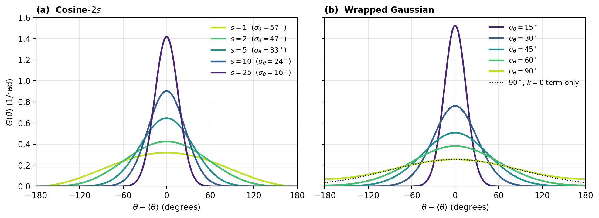
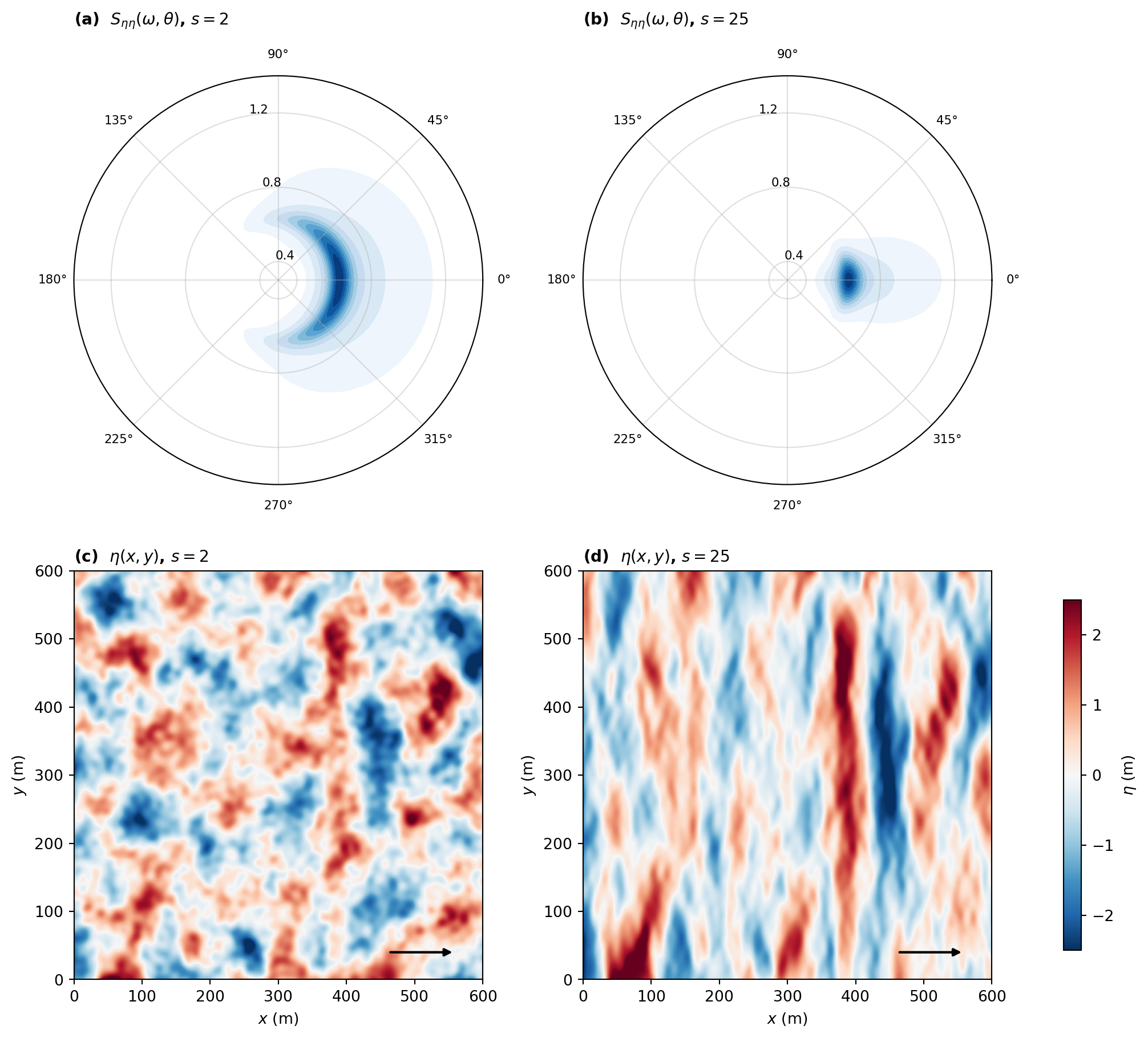
Figure 9.2: **(a)** The cosine-$2s$ spreading function $\eqref{eq-cos-2s-spreading}$, with the circular standard deviation $\sigma_\theta = \sqrt{2/(s+1)}$ of each curve. **(b)** The wrapped Gaussian spreading function $\eqref{eq-wrapped-gaussian-spreading}$. Up to $\sigma_\theta = 45^\circ$ the wrapped curve cannot be told apart from the $k = 0$ term alone. At $\sigma_\theta = 90^\circ$ (dotted: the $k = 0$ term) the plain Gaussian would lose $4.6\%$ of its area beyond $\pm 180^\circ$, and the wrapping returns it.

Figure 9.3 shows what the spreading does to the sea. The JONSWAP spectrum of Figure 9.1(a), with $\gamma = 3.3$, is spread with $s = 2$ and with $s = 25$, and a snapshot of the surface is synthesized from each directional spectrum as a sum of regular waves of all frequencies and directions, $\eta(x, y) = \sum_{m}\sum_{n} a_{mn}\cos\left(k_m x\cos\theta_n + k_m y\sin\theta_n + \varphi_{mn}\right)$, with $a_{mn} = \sqrt{2 S_{\eta\eta}(\omega_m, \theta_n)\,\Delta\omega\,\Delta\theta}$ and $k_m = \omega_m^2/g$. Both have the same frequency spectrum, and hence the same $H_s$, and both use the same random phases $\varphi_{mn}$. Only the spreading differs. With $s = 25$ the crests are long and nearly parallel; with $s = 2$ they are short and the sea is confused.

Figure 9.3: **(a, b)** The directional spectrum $S_{\eta\eta}(\omega, \theta) = S_{\eta\eta}(\omega)G(\theta)$ in polar form (radius: $\omega$ in rad/s; angle: $\theta$), each relative to its own maximum. $S_{\eta\eta}(\omega)$ is the JONSWAP spectrum with $H_s = 4$ m, $T_p = 10$ s and $\gamma = 3.3$, and $G(\theta)$ is the cosine-$2s$ function about $<\theta> = 0$, with $s = 2$ and $s = 25$. **(c, d)** A snapshot of the sea surface synthesized from each spectrum, with the same random phases. The mean direction of travel is $+x$, and the peak wavelength is $2\pi g/\omega_p^2 = 156$ m.

General forms of the spreading function can be derived by letting $<\theta>$, $s$ or $\sigma_\theta$ be a function of frequency.

9.14 Response of a Single Degree of Freedom System

In Chapter 3 we saw that the response of single degree of freedom system to an arbitrary force can be obtained by convolving the force $F(t)$ with the impulse response function of the system $h(t)$.

\[\begin{align} x(t) = \frac{1}{k} \int_{-\infty}^{t} F(\tau)h(t-\tau) d\tau \end{align}\]

Since $h(t-\tau) = 0$ for $t -\tau < 0$ or $\tau > t$, the upper limit of the convolution integral can be replaced with $\infty$ without affecting its value. With a change of variable $\theta = t - \tau$, it can be shown that

\[\begin{align} x(t) &= \frac{1}{k} \int_{-\infty}^{\infty} F(\tau)h(t-\tau) d\tau \nonumber\\ &= \frac{1}{k} \int_{\infty}^{-\infty} F(t-\theta)h(\theta) (-d\theta) \nonumber \\ &= \frac{1}{k} \int_{-\infty}^{\infty} F(t-\theta)h(\theta) d\theta \end{align}\]

Thus, convolving $h$ with $F$ results in the same value as convolving $F$ with $h$.

\[\begin{align} x(t) &= \frac{1}{k} \int_{-\infty}^{\infty} F(\tau)h(t-\tau) d\tau \nonumber \\ &= \frac{1}{k} \int_{-\infty}^{\infty} F(t-\tau)h(\tau) d\tau \end{align}\]

Under the assumption of ergodicity, the autocorrelation of $x(t)$ can be computed as:

\[\begin{align} R_{XX}(\tau) &= E\left[x(t) x(t+\tau)\right] \nonumber \\ &= \lim_{T \rightarrow \infty}\frac{1}{T} \int_{-T/2}^{T/2} x(t) x(t+\tau) dt \equiv <x(t) x(t+\tau)> \end{align}\]

where the operator $<.>$ represents the temporal average. Assuming that $F(t)$ is stationary and ergodic, the autocorrelation can be written as:

\[\begin{align} R_{XX}(\tau) &= <x(t) x(t+\tau)> \nonumber\\ &= \frac{1}{k^2}<\int_{-\infty}^{\infty} \int_{-\infty}^{\infty} h(\tau_1) F(t-\tau_1) h(\tau_2) F(t+\tau-\tau_2) d\tau_1 d\tau_2> \nonumber \\ &= \frac{1}{k^2}\int_{-\infty}^{\infty} \int_{-\infty}^{\infty} h(\tau_1) h(\tau_2) <F(t-\tau_1) F(t+\tau-\tau_2)> d\tau_1 d\tau_2 \nonumber \\ &= \frac{1}{k^2}\int_{-\infty}^{\infty} \int_{-\infty}^{\infty} h(\tau_1) h(\tau_2) R_{FF}(\tau + \tau_1 - \tau_2) d\tau_1 d\tau_2 \end{align}\]

The power spectral density of the response is given by:

\[\begin{align} S_{XX} &(\omega) = \int_{-\infty}^{\infty} R_{XX}(\tau) e^{-i\omega\tau} d\tau \nonumber \\ &= \int_{-\infty}^{\infty} \int_{-\infty}^{\infty} \int_{-\infty}^{\infty} \frac{h(\tau_1)}{k} \frac{h(\tau_2)}{k} R_{FF}(\tau + \tau_1 - \tau_2) d\tau_1 d\tau_2 e^{-i\omega\tau} d\tau \nonumber \\ &= \int_{-\infty}^{\infty} \int_{-\infty}^{\infty} \frac{h(\tau_1)}{k} e^{i\omega\tau_1} \frac{h(\tau_2)}{k} e^{-i\omega\tau_2} \int_{-\infty}^{\infty} R_{FF}(\tau + \tau_1 - \tau_2) e^{-i\omega(\tau+\tau_1-\tau_2)} d\tau d\tau_1 d\tau_2 \nonumber \\ &= \int_{-\infty}^{\infty} \frac{h(\tau_1)}{k} e^{i\omega\tau_1}d\tau_1 \int_{-\infty}^{\infty} \frac{h(\tau_2)}{k} e^{-i\omega\tau_2}d\tau_2S_{FF} (\omega)\nonumber \\ &= \frac{\hat{h}^{*}(\omega)}{k} \frac{\hat{h}(\omega)}{k} S_{FF} (\omega) \nonumber\\ &= \frac{|\hat{h}(\omega)|^2}{k^2} S_{FF} (\omega) \end{align}\]

Thus the response power spectral density can be obtained by multiplying the power spectral density of the input forcing with the square of the RAO of the underlying dynamical system.

Both sides of this relation are even in $\omega$, so it holds equally between the one-sided spectra. The response has zero mean, so its variance is the value of its autocorrelation function at $\tau = 0$, which is the area under its one-sided spectrum:

\[\begin{align} \sigma_x^2 = R_{XX}(0) = \int_0^\infty S_{XX}(\omega)\, d\omega = \frac{1}{k^2}\int_0^\infty |\hat{h}(\omega)|^2 S_{FF}(\omega)\, d\omega \label{eq-sdof-response-variance} \end{align}\]

The standard deviation of the response is therefore fixed by how the force spectrum overlaps $|\hat{h}|^2$. Force at frequencies where $|\hat{h}|$ is large counts for much, and force where $|\hat{h}|$ is small counts for little. If the whole force spectrum lies well below $\omega_n$, then $|\hat{h}| \approx 1$ over it and $\sigma_x \approx \sigma_F/k$: the response is quasi-static, and the spring alone resists the force. If it lies well above $\omega_n$, then $|\hat{h}| \ll 1$, and the mass is too heavy to follow the force. If it covers $\omega_n$, the resonance peak of $|\hat{h}|^2$, of height about $1/(4\zeta^2)$ and half-power width $2\zeta\omega_n$, takes most of the area of $S_{XX}$, and the response oscillates mostly at $\omega_n$, whatever the frequencies of the force.

Interactive: Random Response of an Oscillator

The explorer below drives a spring–mass–damper system with a random force whose one-sided spectrum is band-limited white noise: $S_{FF}(\omega) = S_0$ between $\omega_1$ and $\omega_2$ and zero elsewhere, so that $\sigma_F^2 = S_0(\omega_2 - \omega_1)$. The three stacked panels on the left carry out $\eqref{eq-sdof-response-variance}$ step by step: the force spectrum, multiplied by $|\hat{h}(\omega)|^2/k^2$, gives the response spectrum, and the area under the response spectrum is $\sigma_x^2$.

The force record is synthesized from its spectrum by the random-phase method, as in the earlier explorers. The response is the sum of the steady responses to each component of the force, which is exact for this force. The stiffness is held at $k = 1$ kN/m, so changing $\omega_n$ changes the mass, and the quasi-static response $F/k$ in metres has the same value as the force in kilonewtons. Play animates the oscillator, with the arrow showing the force and the mass moving with $x(t)$ to the scale of the time history beside it. Meanwhile the record is measured from $t = 0$ up to the playhead. The histograms are compared with the Gaussian PDFs whose $\sigma$ is given by the area under each spectrum. The convergence panel shows the standard deviation of the record so far divided by the value from the spectrum.

The band can be set either with the sliders or by dragging it, or one of its edges, in the force or response panel. Dragging in the RAO panel moves $\omega_n$. When the band changes, either the force variance $\sigma_F^2$ or the spectral level $S_0$ is held fixed, as chosen.

Things to try:

Press Play, raise the playback speed, and watch the convergence panel. After about ten minutes of record the ratio for the force is usually within $10\%$ of $1$. The ratio for the response usually needs a record several times longer to settle as closely, because a narrow-band response has a slowly varying envelope, so a record of a given length contains fewer independent samples of it. Lower $\zeta$ to $0.02$ and press New realization a few times to see how long a record a lightly damped system needs.
Hold $\sigma_F^2$ fixed and move a narrow band (width $0.1$ rad/s) from well below $\omega_n$, through it, to well above it. Below, $x(t)$ follows $F(t)/k$ and the amplification $\sigma_x/(\sigma_F/k)$ is close to $1$. Across $\omega_n$ it rises steeply, and above it falls below $1$.
Put the band across $\omega_n$ and widen it with $S_0$ held fixed. $\sigma_F$ keeps growing as $\sqrt{\omega_2 - \omega_1}$, but once the band is several times wider than $2\zeta\omega_n$, $\sigma_x$ hardly changes: the response is set by the force near resonance only. Repeat with $\sigma_F^2$ held fixed: now $S_0$ falls as the band widens, and so does $\sigma_x$.
With a wide band that covers $\omega_n$, halve $\zeta$ from $0.10$ to $0.05$. The peak of $|\hat{h}|^2$ grows by a factor of $4$, but $\sigma_x$ grows by much less. Problem 7 of the exercises explains why.
Compare the zero upcrossing periods $T_z$ of $F$ and $x$ in the table. Whatever the band, $T_z$ of the response moves towards $2\pi/\omega_n$ as the band covers more of the resonance.

Natural frequency, $\omega_n$ (rad/s): 1.00

Damping ratio, $\zeta$: 0.05

Band centre, $(\omega_1 + \omega_2)/2$ (rad/s): 1.00

Band width, $\omega_2 - \omega_1$ (rad/s): 0.80

When the band changes, hold fixed:

Playback speed: 2×

The stiffness is $k = 1$ kN/m. Play measures the record from $t = 0$ up to the playhead: the histograms, the convergence panel and the table include only the part measured so far. Drag along the time history, or the strip below it, to move the playhead.

force $F(t)$ response $x(t)$ $\pm\sigma$ and Gaussian PDF, with $\sigma^2$ the area under the spectrum histogram of the record so far

The oscillator, the force and response records, and their histograms

$S_{FF}(\omega)$ times $|\hat{h}(\omega)|^2/k^2$ gives $S_{XX}(\omega)$, and the area under $S_{XX}$ is $\sigma_x^2$

Standard deviation of the record so far, divided by the value from the spectrum

Statistic	Record so far	From the spectra

9.15 Statistics of the Response in Irregular Waves

The result above is not special to a single degree of freedom system: it holds for any linear system driven by a stationary random input. For a floating structure the input is the wave elevation itself. Chapter 8 gave the RAO of each mode, $\hat{h}_j(\omega) = \hat{\xi}_j(\omega)/A$, the complex amplitude of the response per unit wave amplitude, and its impulse response $h_j(t)$ relates $\eta(t)$ to $\xi_j(t)$ by a convolution. Repeating the derivation above with the wave elevation as the input, and with the factor $1/k$ already contained in $\hat{h}_j$, gives the response spectrum

\[\begin{align} S_{\xi_j\xi_j}(\omega) = |\hat{h}_j(\omega)|^2\, S_{\eta\eta}(\omega) \label{eq-response-spectrum} \end{align}\]

Because $|\hat{h}_j(\omega)|^2$ is even in $\omega$, this holds for the one-sided spectra as well as for the two-sided ones.

The same result follows directly from the complex representation used for regular waves in Chapter 8. Write each wave component of the random-phase sum used in the explorers of this chapter as the real part of a complex exponential:

\[\begin{align} \eta(t) &= \sum_n a_n \cos(\omega_n t + \varphi_n) = \operatorname{Re}\left\{\sum_n \hat{A}_n e^{i\omega_n t}\right\} \nonumber \\ \hat{A}_n &= a_n e^{i\varphi_n}, \qquad a_n = \sqrt{2 S_{\eta\eta}(\omega_n)\Delta\omega} \end{align}\]

The complex amplitude $\hat{A}_n$ carries both the amplitude and the random phase of the component. The structure responds to each component exactly as to a regular wave: its complex response amplitude is the RAO times the complex wave amplitude, and by linearity the responses add:

\[\begin{align} \xi_j(t) = \operatorname{Re}\left\{\sum_n \hat{h}_j(\omega_n)\, \hat{A}_n\, e^{i\omega_n t}\right\} \end{align}\]

There is no need to track phases separately. The multiplication $\hat{h}_j \hat{A}_n$ rotates each component by the phase of the RAO and scales it by its magnitude, and taking the real part at the end gives the actual response. The $n$-th component of the response has the real amplitude $|\hat{h}_j(\omega_n)\hat{A}_n| = |\hat{h}_j(\omega_n)|\, a_n$, so it contributes $\frac{1}{2}|\hat{h}_j|^2 a_n^2 = |\hat{h}_j(\omega_n)|^2 S_{\eta\eta}(\omega_n) \Delta\omega$ to the variance, which is $\eqref{eq-response-spectrum}$. The phase of $\hat{h}_j\hat{A}_n$ is $\varphi_n + \arg\hat{h}_j(\omega_n)$: a random phase shifted by a fixed amount, and still independent of the other components and uniformly distributed. The response is therefore again a sum of many independent random-phase components. The response of a linear system to a stationary Gaussian sea is therefore itself a zero-mean, stationary Gaussian process. Everything in this chapter applies to it unchanged: its Gaussian PDF, its autocorrelation function, and Rice’s results for upcrossings and peaks, all with the moments of the response spectrum

\[\begin{align} m_n^{(\xi)} = \int_0^\infty \omega^n S_{\xi\xi}(\omega)\, d\omega \end{align}\]

Three practical points:

Units. Use the dimensional RAO. A rotational RAO given per unit wave slope must first be multiplied by $k$: $|\hat{\xi}_5/A|^2 = k^2 |\hat{\xi}_5/(kA)|^2$. With $S_{\eta\eta}$ in m²s/rad, a heave spectrum is then in m²s/rad and a pitch spectrum in rad²s/rad.
Rates and periods. With these moments, Rice’s results for the response read exactly as they did for the waves: \[\begin{align} E[N_{+}(\xi_0)] &= \frac{1}{2\pi}\sqrt{\frac{m_2^{(\xi)}}{m_0^{(\xi)}}} \exp\left(-\frac{\xi_0^2}{2 m_0^{(\xi)}}\right) \nonumber \\ E[N_p] &= \frac{1}{2\pi}\sqrt{\frac{m_4^{(\xi)}}{m_2^{(\xi)}}} \nonumber \\ T_z &= 2\pi\sqrt{\frac{m_0^{(\xi)}}{m_2^{(\xi)}}} \end{align}\]
Velocity and acceleration. Differentiating each component multiplies its amplitude by $\omega$, so the spectra of the velocity and acceleration are \[\begin{align} S_{\dot{\xi}\dot{\xi}}(\omega) = \omega^2 S_{\xi\xi}(\omega), \qquad S_{\ddot{\xi}\ddot{\xi}}(\omega) = \omega^4 S_{\xi\xi}(\omega) \end{align}\] and their variances are $m_2^{(\xi)}$ and $m_4^{(\xi)}$. The fourth moment of the wave spectrum does not exist, because $\omega^4 S_{\eta\eta}(\omega) \propto \omega^{-1}$ at high frequency. The fourth moment of the response spectrum is usually finite, because the RAO falls away in short waves (Chapter 8) and $\omega^4 |\hat{h}_j|^2 S_{\eta\eta}$ then decays fast enough to integrate.

In a short-crested sea the wave components come from many directions, and components from different directions are independent. Their contributions to the variance add, and the response spectrum becomes $S_{\xi\xi}(\omega) = \int_{-\pi}^{\pi} |\hat{h}(\omega, \theta)|^2 S_{\eta\eta}(\omega, \theta)\, d\theta$, with the RAO evaluated for each wave direction relative to the structure.

Short-Term Statistics of the Response

For one sea state, the statistics of the response follow from $m_0^{(\xi)}$, $m_2^{(\xi)}$ and $m_4^{(\xi)}$ exactly as those of the wave elevation did. If the response spectrum is narrow banded (check $\varepsilon$), its amplitudes are Rayleigh distributed and

the standard deviation is $\sigma_\xi = \sqrt{m_0^{(\xi)}}$;
the significant amplitude is $\xi_{1/3} = 2\sqrt{m_0^{(\xi)}}$, and the significant double amplitude (crest to trough) is $4\sqrt{m_0^{(\xi)}}$, the counterpart of $H_s$; the mean amplitude and the mean of the highest tenth are $1.25\sqrt{m_0^{(\xi)}}$ and $2.55\sqrt{m_0^{(\xi)}}$;
the probability that a given response amplitude exceeds $\xi_0$ is $\exp\left(-\xi_0^2/(2 m_0^{(\xi)})\right)$;
the expected number of times the response exceeds $\xi_0$ in a sea state of duration $T_d$ is $E[N_{+}(\xi_0)]\, T_d$. When such exceedances are rare they occur practically independently of each other, and the probability that $\xi_0$ is exceeded at least once is approximately $1 - \exp\left(-E[N_{+}(\xi_0)]\, T_d\right)$;
in $N = T_d/T_z$ oscillations, the level exceeded on average once is found from $N \exp\left(-\xi_N^2/(2m_0^{(\xi)})\right) = 1$: \[\begin{align} \xi_N = \sqrt{2 m_0^{(\xi)} \ln N} \label{eq-response-extreme} \end{align}\] For large $N$ this is close to the most probable largest amplitude in the sea state. For example, a 3 hour sea state with $T_z = 10$ s has $N \approx 1080$ oscillations and $\xi_N \approx 3.7\sigma_\xi$, about $1.9$ times the significant amplitude.

These are the same formulas as for the waves, because the response is a Gaussian process of the same kind. What changes is the spectrum. The RAO acts as a filter: it amplifies the waves near the resonance of the structure and suppresses those it does not feel. The response spectrum is therefore often narrower than the wave spectrum, and its mean period can be quite different.

Response at Forward Speed: the Encounter Spectrum

Everything so far assumed a structure at rest, which meets each wave component at its own frequency $\omega$. A ship with forward speed $U$ meets the component of frequency $\omega$ at the encounter frequency (Chapter 7)

\[\begin{align} \omega_e = \omega - \frac{\omega^2 U}{g}\cos\beta \label{eq-encounter-frequency-spectrum} \end{align}\]

and its RAOs are computed at $\omega_e$ (Chapter 8). The wave elevation recorded by a probe moving with the ship is made of the same components as the sea, with the same amplitudes and random phases, but each component now oscillates at $\omega_e$. The sea as seen from the ship is therefore described by an encounter spectrum $S^{e}_{\eta\eta}(\omega_e)$. It follows from the fact that the components in a band $d\omega$ carry the same energy whatever frequency they are labelled with:

\[\begin{align} S^{e}_{\eta\eta}(\omega_e)\, |d\omega_e| &= S_{\eta\eta}(\omega)\, d\omega \nonumber \\ \Rightarrow \quad S^{e}_{\eta\eta}(\omega_e) &= \frac{S_{\eta\eta}(\omega)}{\left|d\omega_e/d\omega\right|} = \frac{S_{\eta\eta}(\omega)}{\left|1 - 2\omega U\cos\beta/g\right|} \label{eq-encounter-spectrum} \end{align}\]

The area under the spectrum is unchanged, so the encounter spectrum has the same $m_0$ and the same $H_s$ as the sea. Only the frequencies are relabelled, and the explorer at the end of this section shows how differently that works out in head and in following seas:

Head and beam seas ($\cos\beta \leq 0$). The encounter frequency rises monotonically with $\omega$, so each $\omega_e$ comes from exactly one wave frequency. In head seas the spectrum moves to higher frequencies and spreads out, and its peak drops to keep the area the same: the ship meets the waves more often.
Following and quartering seas ($\cos\beta > 0$). The encounter frequency rises to a maximum $\omega_{e,\max} = g/(4U\cos\beta)$ at $\omega = g/(2U\cos\beta)$, where $d\omega_e/d\omega = 0$, and then falls. It passes through zero at $\omega = g/(U\cos\beta)$, the wave whose phase speed equals the ship’s speed along its direction, and becomes negative for shorter waves, which the ship overtakes. A component with negative $\omega_e$ oscillates at $|\omega_e|$. Up to three wave frequencies therefore meet the ship at the same $|\omega_e|$, and their contributions must be added: \[\begin{align} S^{e}_{\eta\eta}(\omega_e) = \sum_{i} \frac{S_{\eta\eta}(\omega_i)}{\left|1 - 2\omega_i U\cos\beta/g\right|}, \qquad |\omega_e(\omega_i)| = \omega_e \end{align}\] The density is infinite at $\omega_{e,\max}$, but the singularity is integrable and $m_0$ is still finite.

The response spectrum at forward speed is the encounter spectrum multiplied by the squared RAO, $S^{e}_{\xi_j\xi_j}(\omega_e) = |\hat{h}_j|^2 S^{e}_{\eta\eta}(\omega_e)$, with the RAO of each branch in following seas. Its moments are taken with respect to the frequency at which the response actually oscillates, $|\omega_e|$. They are most easily computed by changing the variable of integration back to the wave frequency, which removes the Jacobian $|d\omega_e/d\omega|$ and with it the singularity and the bookkeeping of branches:

\[\begin{align} m_n^{(\xi)} = \int_0^\infty \omega_e^n\, S^{e}_{\xi_j\xi_j}(\omega_e)\, d\omega_e = \int_0^\infty |\omega_e(\omega)|^n\, |\hat{h}_j(\omega)|^2\, S_{\eta\eta}(\omega)\, d\omega \label{eq-encounter-moments} \end{align}\]

where $\hat{h}_j(\omega)$ is the RAO for the wave component of frequency $\omega$, evaluated at its encounter frequency. The short-term statistics above then apply unchanged with these moments. In particular, the velocity and acceleration of the response carry $\omega_e^2$ and $\omega_e^4$, not $\omega^2$ and $\omega^4$. In head seas, where $\omega_e > \omega$, forward speed therefore makes the accelerations larger relative to the displacements.

The higher moments of the encountered wave elevation itself are worth a caution. In head seas $\omega_e$ grows like $\omega^2$ in short waves, so $\omega_e^2 S_{\eta\eta}(\omega)$ decays only like $\omega^{-1}$ and even $m_2$ of the encounter spectrum depends on the cut-off frequency. A response does not have this difficulty as long as its RAO falls away in short waves.

Interactive: Response of the KCS in Irregular Waves

The explorer below puts the whole chapter to work on the KCS, the benchmark ship of the earlier chapters. Choose a sea state, a speed and heading of the ship, and a response. The explorer then carries out every step of this section:

The sea. It builds the Pierson–Moskowitz or JONSWAP spectrum $\eqref{eq-pierson-moskowitz}$, $\eqref{eq-jonswap}$ for the chosen $H_s$ and $T_p$, and converts it to the encounter spectrum $S^{e}_{\eta\eta}(\omega_e)$ seen by the ship $\eqref{eq-encounter-spectrum}$.
The RAO. It solves the six coupled equations of motion of Chapter 8 at every frequency, with the HydRA coefficients and loads of the motion RAO explorer (mesh residual removed) and the viscous roll damping $\zeta_v$, and multiplies the RAO by $i\omega_e$ or $-\omega_e^2$ for the velocity or the acceleration.
The response spectrum. It multiplies $|\hat{h}|^2$ by the spectrum $\eqref{eq-response-spectrum}$, and computes its moments by integrating over the wave frequency $\eqref{eq-encounter-moments}$.
The statistics. It evaluates the short-term statistics of the response from $m_0$, $m_2$ and $m_4$.
A record. It synthesizes a 3 hour record of the encountered wave and of the response as $\operatorname{Re}\{\sum_n \hat{h}(\omega_n)\hat{A}_n e^{i\omega_{e,n} t}\}$, and measures the same statistics from it, so that the prediction and the “measurement” can be compared side by side.

The three panels of spectra can be drawn against the encounter frequency $\omega_e$, where the response actually oscillates, or against the wave frequency $\omega$. Against $\omega$, each point belongs to one wave component and nothing folds, and the area under the bottom panel is again $m_0$ of the response. That is the form in which the moments are computed.

Two limits of the data apply. First, the RAOs are used only up to $\omega = 1.0$ rad/s, a wavelength of $62$ m or about $L_{pp}/4$, and are tapered to zero from $0.9$ rad/s, as in the impulse response explorer of Chapter 8. At forward speed the HydRA results above this frequency are not reliable, and in head and bow seas waves this short hardly move the KCS. Left in, the spurious short-wave data would add energy where there should be almost none, and the factor $\omega_e^4$ of an acceleration would magnify it. In beam seas, where a wave runs across the beam rather than the length, the cut also removes a little genuine heave and roll. Second, as $\omega_e \rightarrow 0$ in following and quartering seas the linear equations of motion break down (Chapter 8): sway and yaw have no restoring force, and at $24$ kn in stern quartering seas the solver returns a spurious roll response near $\omega_e = 0$ that would dominate everything else. Wave components that the ship meets with $|\omega_e| < 0.08$ rad/s, an encounter period of more than $78$ s, are therefore left out.

Things to try (values for the default sea, a Pierson–Moskowitz spectrum with $H_s = 4$ m and $T_p = 10$ s, and $\zeta_v = 0.05$):

Speed raises accelerations more than motions. In head seas, going from $0$ to $24$ kn raises the standard deviation of heave only from $0.24$ m to $0.30$ m, but that of the heave acceleration from $0.10$ to $0.20$ m/s². The encounter spectrum moves to higher frequencies, its mean zero upcrossing period of heave drops from $9.8$ s to $8.0$ s, and the $\omega_e^4$ of the acceleration does the rest. Pitch acceleration behaves the same way.
Following seas fold the spectrum. At $24$ kn in following seas the whole sea is squeezed below $\omega_{e,\max} = g/(4U\cos\beta)$. The ship meets the waves so slowly that the heave has a zero upcrossing period of about $38$ s, more than five times that of the waves ($7.1$ s). Compare the spectra drawn against $\omega$ and against $\omega_e$.
Roll in stern quartering seas. In beam seas at zero speed the KCS hardly rolls ($\sigma \approx 0.14^\circ$), because its roll natural period of about $39$ s is far from the energy of the sea. At $24$ kn in stern quartering seas ($\beta = 45^\circ$) the ship meets $7$ s waves at the roll natural frequency (Chapter 8). The standard deviation of roll grows to about $8^\circ$, with $T_z \approx 34$ s, and the largest roll expected in 3 hours is about $28^\circ$, far beyond the range in which linear theory can be trusted. Change $\zeta_v$: doubling the damping to $0.10$ lowers $\sigma$ only to about $6^\circ$. This synchronous rolling, with the encounter period of the waves tuned to the roll natural period, is one of the dangers in following and quartering seas that the IMO guidance to masters, MSC.1/Circ.1228, warns against.
The ship in beam seas follows the long waves. At zero speed in beam seas, the heave has nearly the same standard deviation as the wave elevation, about $1$ m: its RAO is close to one over most of the spectrum.
Prediction against measurement. In every case the standard deviation and the zero upcrossing period of the 3 hour record agree with the spectrum to within a few per cent. The number of upcrossings of the threshold and the largest value scatter more, as statistics of rare events do. Press New realization to see by how much.

Sea

Speed

Heading

Response

Plot against

Significant wave height, $H_s$ (m): 4.0

Peak period, $T_p$ (s): 10.0

JONSWAP peak factor, $\gamma$: 3.3

Viscous roll damping, $\zeta_v$: 0.05

Threshold, $\xi_0 / \sigma$: 2.0

Playback speed: 5×

Rotations are in degrees. Heave, roll and pitch are the motions of the BCS origin at midship. The record is 3 hours long; Play scrolls the 120 s window through it, and the strip below the record moves the window by dragging. The histogram and the table use the whole record.

From top to bottom: the sea, the squared RAO of the chosen response, and their product, the response spectrum

The wave elevation met by the ship at its origin, $\eta_e(t)$, and the response, with upcrossings of the threshold $\xi_0$ (triangles) and the histogram of the whole record against the Gaussian PDF of the spectrum (dashed)

Statistic	From the spectrum	From the 3 h record

9.16 Exercises

Throughout, $S_{\eta\eta}(\omega)$ is the one-sided spectrum of the circular frequency $\omega$, in m$^2$s/rad, and $m_n = \int_0^\infty \omega^n S_{\eta\eta}(\omega)\,d\omega$, unless a problem says otherwise. “PM” is the Pierson–Moskowitz spectrum $\eqref{eq-pierson-moskowitz}$ and “JONSWAP” the spectrum $\eqref{eq-jonswap}$, both in their $H_s$, $T_p$ form. The sea is long-crested and the water deep. Every process is zero-mean, stationary and Gaussian, unless a problem asks you to question exactly that. Use $g = 9.81$ m/s$^2$.

Every problem can be answered with the results of this chapter: the stochastic process and its ensemble, stationarity and ergodicity, the autocorrelation function and the spectrum, Rice’s results for crossings and peaks, the wave spectra, and the response spectrum with its short-term statistics. Results from Chapter 2 (the dynamic amplification factor), Chapter 3 (Fourier transform pairs), Chapter 7 (the encounter frequency) and Chapter 8 (the RAO and its meaning) are used freely.

This is the first set of problems in which neither the sea nor the response is known in advance. Only their statistics are. A regular wave has one amplitude and one period; a sea state has a distribution of both, and the questions change accordingly. One no longer asks “how large is the response?” but “how large is it likely to be, how often, and how sure can we be from one record?”

A note on what is being tested. As in Chapter 8, most problems are built around a statement that is almost right: “a longer record gives a smoother spectrum”, “the bandwidth measures how much energy lies at high frequencies”, “the most probable maximum is a safe design value”, “rogue waves prove that linear theory fails”, “halving the damping doubles the resonant response”, “a JONSWAP sea is always more severe than a Pierson–Moskowitz sea of the same $H_s$ and $T_p$”, “in following seas the ship meets every wave slowly, so it simply rides them”. Each survives a casual check and fails a careful one. Where a problem asks why, a number alone earns nothing.

The structures and sea states these problems refer to

Three sea states recur below, all described by the Pierson–Moskowitz spectrum:

	$H_s$ (m)	$T_p$ (s)	$\omega_p$ (rad/s)
the reference sea (the default of the explorers of this chapter)	$4$	$10$	$0.628$
the storm	$14$	$16$	$0.393$
the swell	$3$	$22$	$0.286$

A real swell has a narrower spectrum than the Pierson–Moskowitz form, which is used here for simplicity.

Two floating bodies return from the exercises of Chapter 8, both with a heave damping ratio $\zeta = 0.05$ and the same heave natural frequency $\omega_n = 0.2577$ rad/s ($T_n = 24.4$ s). The spar buoy with a heave plate (a column of $8$ m diameter to $20$ m depth, on a disc of $24$ m diameter and $4$ m thickness) has the heave RAO \[\hat h_b(\omega) = \frac{e^{-kd}\left[A_c - A_p\left(1 - e^{-kh}\right)\right] - (A_{33}/\rho)\,k\,e^{-kd_c}}{A_c\left[1 - (\omega/\omega_n)^2 + 2i\zeta\,\omega/\omega_n\right]},\] with $k = \omega^2/g$, $d = 20$ m, $h = 4$ m, $d_c = 22$ m, $A_c = 50.27$ m$^2$, $A_p = 452.4$ m$^2$ and $A_{33}/\rho = 4608$ m$^3$. The classic spar is a plain column of the same diameter and of draft $d = g/\omega_n^2 = 147.7$ m, with added mass neglected: \[\hat h_c(\omega) = \frac{e^{-kd}}{1 - (\omega/\omega_n)^2 + 2i\zeta\,\omega/\omega_n}.\]

Where the KCS appears, the numbers quoted come from the response explorer of this chapter or from the data at the start of the exercises of Chapter 8. Figure 9.4 shows the three spectra and the two RAOs.

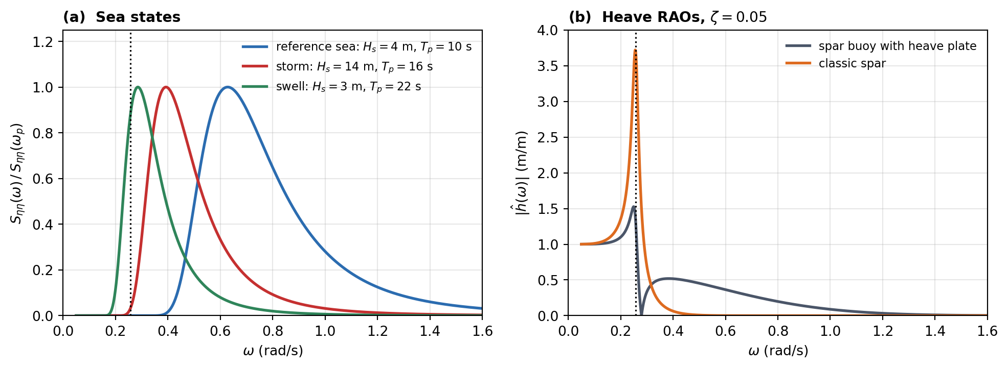
Figure 9.4: **(a)** The three sea states of these problems, each drawn relative to its own peak value. The swell peaks close to the heave natural frequency of the two spars (dotted line), the storm well above it, and the reference sea far above it. **(b)** The magnitude of the heave RAOs of the two spars. Both resonate at $T_n = 24.4$ s. The classic spar is quiet at every shorter period. The buoy has a smaller resonant peak and a zero just above $\omega_n$, but an RAO of about $0.4$ to $0.5$ from $12$ to $20$ s.

What one record can tell you: stationarity, ergodicity and the Gaussian assumption.
1. A single wave component with a random phase, $\eta(t) = a\cos(\omega_0t + \varphi)$, has $a$ and $\omega_0$ fixed and $\varphi$ uniformly distributed on $[0, 2\pi)$. Show that it is stationary, and find its mean and its autocorrelation function. Show that the time averages of $\eta$ and $\eta^2$ over any one realization equal the ensemble averages. Find the PDF of $\eta_t$ and its kurtosis $E[\eta^4]/E[\eta^2]^2$, which is $3$ for a Gaussian variable. Is the process Gaussian? If $\varphi$ were uniform on $[0, \pi)$ only, would the process still be stationary?
2. The explorers of this chapter synthesize the sea as $\eta(t) = \sum_n a_n\cos(\omega_nt + \varphi_n)$, with fixed amplitudes $a_n = \sqrt{2S_{\eta\eta}(\omega_n)\Delta\omega}$, distinct frequencies and independent uniform phases. Find $R_{\eta\eta}(\tau)$. Show that the mean square of one realization, taken over a long record, is $\sum_na_n^2/2$ whatever the phases, so that every realization has exactly the same variance. Show that the kurtosis is $3 - \tfrac{3}{8}\sum_na_n^4/\sigma^4$, with $\sigma^2 = \sum_na_n^2/2$. For $N$ components of equal amplitude, how many are needed to bring the kurtosis within $1\%$ of the Gaussian value? What is then the largest elevation the model can ever produce, in units of $\sigma$? Is the model Gaussian?
3. Now let the amplitudes be random instead: $\eta(t) = \sum_n\left(A_n\cos\omega_nt + B_n\sin\omega_nt\right)$, with all $A_n$ and $B_n$ independent and Gaussian, of zero mean and variance $a_n^2/2$. Show that the process is exactly Gaussian, stationary, and has the same $R_{\eta\eta}(\tau)$ as in (b). Show that the long-time mean square of one realization is now a random variable, and find its coefficient of variation for $N$ components of equal variance. Which of the two models is ergodic in the mean square, and which is Gaussian? Which better imitates a record measured at sea, and when does the difference matter?
4. A wave buoy records without a break for a year, at a site where $H_s$ is $1$, $2$, $4$ and $8$ m for $50$, $30$, $15$ and $5\%$ of the time. Each sea state is stationary and Gaussian. Is the year-long record stationary? A student computes “the significant wave height of the year” as $4\sqrt{m_0}$ from the variance of the whole record. Find it, compare it with the mean $H_s$, and explain why it is the $H_s$ of no sea state at all. Find the kurtosis of the elevation over the year. Use the year’s variance in a Gaussian model to find the probability that $|\eta|$ exceeds three standard deviations, and compare it with the true probability. What does this say about how long-term statistics must be built?
5. A model of a floating platform is tested in a wave basin. To obtain “ensemble averages”, the wavemaker plays the same $30$-minute signal ten times, and the standard deviation and the largest value of the motion are averaged over the ten runs. What has actually been averaged? What can the ten runs tell you, and what can they not? How should the test be run instead?
The autocorrelation function: what it can be, and what it says.
1. Which of the following can be the autocorrelation function of a stationary process?
  1. $R(\tau) = \sigma^2e^{-|\tau|/\tau_c}$
  2. $R(\tau) = \sigma^2e^{-\tau^2/(2\tau_c^2)}\cos\omega_0\tau$
  3. $R(\tau) = \sigma^2$ for $|\tau| \le T_0$ and zero otherwise
  4. $R(\tau) = \sigma^2(1 - |\tau|/T_0)$ for $|\tau| \le T_0$ and zero otherwise
  5. $R(\tau) = \sigma^2e^{-|\tau|/\tau_c}(1 + |\tau|/\tau_c)$
  All five are even and largest at $\tau = 0$. For (iii), consider the covariance matrix of $\eta$ at the times $0$, $0.6T_0$ and $1.2T_0$. Which property, beyond evenness and $|R(\tau)| \le R(0)$, must an autocorrelation function have?
2. For a zero-mean stationary Gaussian process, show from the joint PDF that, given $\eta_t = x$, $\eta_{t+\tau}$ is Gaussian with mean $\rho_{\eta\eta}(\tau)\,x$ and variance $m_0\left(1 - \rho_{\eta\eta}^2(\tau)\right)$. In the reference sea, $\rho_{\eta\eta}(4\ \text{s}) = -0.653$, its most negative value. An observer sees the elevation at $+3$ m. Find the expected elevation $4$ s later, its standard deviation, and the probability that it is below $-2$ m. Compare with the unconditional probability. In a narrow band sea, what would the elevation half a period later be, and why is the answer here so different?
3. With $R_{\eta\eta}(\tau) = \int_0^\infty S_{\eta\eta}(\omega)\cos\omega\tau\,d\omega$, show that $E[\eta\dot\eta] = R'(0) = 0$, $E[\dot\eta^2] = -R''(0) = m_2$, $E[\eta\ddot\eta] = R''(0) = -m_2$ and $E[\ddot\eta^2] = R''''(0) = m_4$, all at the same instant. Hence show that at any instant the elevation and its rate of change are independent, and that the correlation coefficient between $\eta$ and $\ddot\eta$ is $-\sqrt{1 - \varepsilon^2}$. What does this say about a narrow band process, and why are all its maxima positive? Use the result to explain what the bandwidth $\varepsilon$ actually measures.
4. In a short time $dt$, the process upcrosses the level $\eta_0$ if $\dot\eta > 0$ and $\eta_0 - \dot\eta\,dt < \eta < \eta_0$. Show that the expected rate of upcrossings is $\int_0^\infty v\,p_{\eta\dot\eta}(\eta_0, v)\,dv$, and use (c) to recover Rice’s result. Why does the rate of upcrossings need $m_2$, while the rate of peaks needs $m_4$? For the processes (i) and (v) of part (a), find the spectrum, the zero upcrossing rate and the rate of peaks. Which of the five could describe the elevation of the sea surface?
5. A spectrum concentrated at one frequency, $S_{\eta\eta} = m_0\delta(\omega - \omega_0)$, gives $R_{\eta\eta}(\tau) = m_0\cos\omega_0\tau$, which never decays. Show that this process can be predicted for all future time from $\eta$ and $\dot\eta$ at one instant. A spectrum of Gaussian shape about $\omega_0$, with standard deviation $s \ll \omega_0$, gives $\rho_{\eta\eta}(\tau) \approx e^{-s^2\tau^2/2}\cos\omega_0\tau$. Writing the process as a carrier at $\omega_0$ under a slowly varying envelope, argue that the error variance of the best prediction from $\eta$ and $\dot\eta$ at $t$ is about $m_0\left(1 - e^{-s^2\tau^2}\right)$. With $\omega_0 = 0.5$ rad/s and $s = 0.05$ rad/s, how many wave periods ahead is the prediction error half the variance of the sea? What does this imply for predicting the motion of a vessel from a wave probe on board (Problem 8(d) of Chapter 8)?
One sea, four numbers: spectral conventions and the periodogram.
1. For the reference sea, find the peak value of
  1. the one-sided $S_{\eta\eta}(\omega)$ of this book,
  2. $S_{\eta\eta}(f)$,
  3. the two-sided $S^{(2)}_{\eta\eta}(\omega)$ of this book, the Fourier transform of $R_{\eta\eta}$,
  4. a two-sided spectrum in $f$ normalised so that its integral over $-\infty < f < \infty$ is $m_0$, and
  5. a two-sided spectrum in $\omega$ normalised so that its integral over $-\infty < \omega < \infty$ is $m_0$.
  Give the units. Two of these are numerically equal: show why. A report quotes a peak spectral density of $7.16$ without units, and a reader takes it as $S_{\eta\eta}(\omega)$ of a PM spectrum with $T_p = 10$ s. What $H_s$ does the reader infer? What if the report had said $14.3$?
2. A record of length $T$ of a Gaussian sea is the random-amplitude sum of Problem 1(c), with $\omega_n = 2\pi n/T$. Show that its periodogram at $\omega_k$ is $\tfrac{T}{4}\left(A_k^2 + B_k^2\right)$, that its expected value is $S^{(2)}_{\eta\eta}(\omega_k)$, and that its ratio to the expected value is exponentially distributed with mean one and standard deviation one, whatever $T$ is. Find the probability that a periodogram ordinate is below $10\%$ of the true spectrum, and that it is above three times the true spectrum. A student doubles the length of the record “to make the spectrum converge”. What happens to the scatter, and what improves instead?
3. Averaging the periodograms of $K$ independent segments of length $T/K$ (Welch’s method without overlap) gives ordinates distributed as $\chi^2_{2K}/(2K)$, with a coefficient of variation of $1/\sqrt K$ and a frequency resolution of $2\pi K/T$. For a $3$ hour record, choose $K$ to make the coefficient of variation $20\%$, and find the resolution. Is it fine enough to resolve the peak of the reference sea, whose half-power width you should compute, and the resonant peak of the classic spar’s heave spectrum in the swell, whose half-power width is about $2\zeta\omega_n$? How long a record would give a $20\%$ scatter with at least four ordinates across the spar’s resonant peak? Why does a model test of a lightly damped structure need longer records than a test of a well damped one?
4. A record synthesized as in Problem 1(b), with fixed amplitudes and random phases on the frequencies $\omega_k = 2\pi k/T$, is analysed over its full length $T$. Its periodogram equals the target spectrum exactly at every $\omega_k$. A student concludes that the periodogram is a perfect estimator, at least for simulated data. Explain what is wrong with the conclusion.
5. In deriving the periodogram, this chapter estimates the autocorrelation as $R^T_{\eta\eta}(\tau) = \frac{1}{T}\int\eta_T(t)\eta_T(t + \tau)\,dt$, dividing by the full length $T$, while the explorer divides the sum of products by the number of pairs, $N - k$. Show that the expected value of the first is $(1 - |\tau|/T)R_{\eta\eta}(\tau)$, so that it is biased, while the second is unbiased. Show that the Fourier transform of the first is exactly the periodogram, and hence never negative. Explain why the Fourier transform of the unbiased estimate can be negative at some frequencies, and why its values at lags comparable with $T$ are useless anyway.
Counting waves: upcrossings, peaks and the bandwidth.
1. A spectrum is made of two lines: a fraction $1 - p$ of the variance at $\omega_1$ and a fraction $p$ at $5\omega_1$, much as in the upcrossings and peaks explorer. Show that $1 - \varepsilon^2 = (1 + 24p)^2/(1 + 624p)$. Find the values of $p$ that give $\varepsilon = 0.9$, and compare the smaller one with the explorer’s statement that about $1.3\%$ of the variance in the secondary peak gives $\varepsilon = 0.9$. What is the largest bandwidth this family can have, and at what $p$? Is $\varepsilon$ a measure of how much of the energy lies at high frequencies?
2. For both values of $p$ with $\varepsilon = 0.9$, find the zero upcrossing rate and the peak rate relative to their values with $p = 0$, the number of peaks per zero upcrossing, and the fraction of negative peaks, $(1 - \sqrt{1 - \varepsilon^2})/2$. Rice’s PDF of the peaks depends only on $m_0$ and $\varepsilon$. Do the two processes then have the same distribution of peaks? Sketch a few periods of each. What in a record would tell them apart?
3. The Pierson–Moskowitz spectrum has no $m_4$, so $\varepsilon$ depends on the cut-off frequency $\omega_c$ (callout above). With the substitution $u = \tfrac54(\omega_p/\omega)^4$, show that for $\omega_c \gg \omega_p$ \[m_4(\omega_c) \approx 5m_0\omega_p^4\left[\ln\frac{\omega_c}{\omega_p} - \frac{\gamma_E + \ln(5/4)}{4}\right],\] with $\gamma_E = 0.5772$ and $\int_x^\infty e^{-u}u^{-1}du \approx -\gamma_E - \ln x$ for small $x$. Show also that $m_2(\infty) = \frac{\sqrt{5\pi}}{2}\,m_0\omega_p^2$, and that truncating at $\omega_c$ removes about $\frac{5}{2}m_0\omega_p^4/\omega_c^2$ from it. Reproduce the values $\varepsilon = 0.59$, $0.71$ and $0.80$ of the callout for cut-offs at $3$, $5$ and $10\,\omega_p$. Where must the cut-off lie for $\varepsilon = 0.9$, and what is the length of the waves there?
4. The reference sea is measured by a wave buoy that cannot follow waves above $0.5$ Hz, and by a laser altimeter that resolves waves up to $2$ Hz. Assume that the Pierson–Moskowitz form holds up to both limits. For each instrument, find the expected numbers of zero upcrossings and of peaks in a $20$ minute record. How many waves are there in the record?
5. Explain why wave statistics are based on zero upcrossing waves, each wave running from one zero upcrossing to the next, and not on all the peaks of the record. In the explorer, as $\varepsilon$ grows, the mean of the highest third of all peaks falls well below $2\sqrt{m_0}$, while $H_{1/3}$ of the zero upcrossing waves stays close to $4\sqrt{m_0}$. Explain both observations.
The largest wave in a storm. On 1 January 1995, the Draupner E platform in the North Sea recorded a wave of height $25.6$ m, with a crest $18.5$ m above the mean water level, in a sea state with $H_s \approx 12$ m. Take the storm to have $H_s = 12$ m and $T_z = 11$ s, and to last $3$ hours. Assume a narrow band sea except in (d).
1. Show that the wave heights $H = 2a$ satisfy $P(H > h) = \exp(-2h^2/H_s^2)$. Find the mean height, the root mean square height and $H_{1/10}$ in terms of $H_s$, and the number of waves $N$ in the storm.
2. The most probable largest height in $N$ waves is close to the height exceeded on average once, $H_{\text{mp}} = H_s\sqrt{\ln N/2}$. Show that the probability that the largest of $N$ independent waves exceeds it is $1 - (1 - 1/N)^N \approx 1 - e^{-1}$. A designer adopts the “most probable maximum” as the design wave height, on the grounds that it is the single most likely value. Comment. Find the height that the largest wave exceeds with a probability of $10\%$, and of $1\%$. How does the Draupner wave compare?
3. A rogue wave is commonly defined as one with $H > 2H_s$. Find the probability that a given wave is a rogue wave, the expected number of rogue waves in the storm, and the probability that there is at least one. Does a rogue wave, so defined, show that linear theory has failed? Now do the same for the Draupner crest: find the probability that a crest of a Gaussian sea exceeds $18.5$ m in this storm, and how long one would wait, in storms like this one, to see it once. What has failed, and in which direction does the failure go?
4. The narrow band model takes every trough to be as deep as the preceding crest is high. Following Næss, a better estimate of the height distribution is $P(H > h) = \exp\left[-h^2/\left(4m_0(1 - \rho_{\min})\right)\right]$, where $\rho_{\min}$ is the most negative value of $\rho_{\eta\eta}(\tau)$, at about half a period. Check that this reduces to (a) for a narrow band sea. With $\rho_{\min} = -0.653$, the value for a Pierson–Moskowitz spectrum (Problem 2(b)), find $H_{1/3}$ in units of $\sqrt{m_0}$ and the most probable largest height in the storm. Field measurements give $H_{1/3} \approx 3.8\sqrt{m_0}$. Is the narrow band model conservative?
5. By how much does $H_{\text{mp}}$ grow if the storm lasts $6$ hours instead of $3$? A platform designer wants the largest wave in a $25$-year life, and proposes to put $N = 25\ \text{years}/T_z$ into the formula of (b), with $H_s = 12$ m. What is wrong with this, and what is needed instead?
What $H_s$, $T_p$ and $\gamma$ fix, and what they do not.
1. Show that the Pierson–Moskowitz spectrum peaks at $\omega_p$ with $S_{\eta\eta}(\omega_p) = \tfrac{5}{16}H_s^2e^{-5/4}/\omega_p$. Using the result for $m_2$ of Problem 4(c), show that $T_z = (4/(5\pi))^{1/4}\,T_p = 0.710\,T_p$. A wave buoy reports $H_s = 4$ m and $T_z = 7.1$ s. What $T_p$ should you use for a Pierson–Moskowitz spectrum? For a JONSWAP spectrum with $\gamma = 3.3$, for which $T_z/T_p = 0.777$, what $T_p$ should you use, and what is the peak spectral density? Why must a mean period be converted with the spectral shape in mind?
2. Show that a sea with $T_p = 5\sqrt{H_s}$ has a steepness $2\pi H_s/(gT_p^2)$ that does not depend on $H_s$, and evaluate it. A sea with $H_s = 4$ m has $T_p = 7$ s, $8$ s or $10$ s. For each, find the steepness and the value of $\gamma$ recommended by DNV-RP-C205. Which of them are still growing?
3. Compare a JONSWAP spectrum with $\gamma = 3.3$ and a Pierson–Moskowitz spectrum with the same $H_s$ and $T_p$. Show that their peak values are in the ratio $A_\gamma\gamma$, and evaluate it. A lightly damped structure with natural frequency $\omega_n$ responds, to a good approximation, with a variance proportional to $S_{\eta\eta}(\omega_n)$ (Problem 7). Find the ratio of the standard deviations of its response in the two spectra for $\omega_n = 0.9\omega_p$, $\omega_p$ and $1.3\omega_p$. Is the JONSWAP spectrum always the conservative choice?
4. For the cosine spreading function $\eqref{eq-cos-2s-spreading}$ with $s = 1$ and mean direction $\langle\theta\rangle = 0$, show that $G(\theta) = (1 + \cos\theta)/(2\pi)$ and that it integrates to one. What fraction of the wave energy then travels against the mean direction? For this family, $E[\cos\theta] = s/(s + 1)$ and $E[\cos2\theta] = s(s - 1)/[(s + 1)(s + 2)]$. In long-crested head seas a ship symmetric about its centreplane cannot roll (Problem 6(a) of Chapter 8). Model its roll RAO in other headings as $|\hat h_4(\omega, \beta)|^2 = |\hat h_4(\omega, 90^\circ)|^2\sin^2\beta$. Show that the roll variance in a short-crested sea whose mean direction is head seas is $E[\sin^2\theta] = \tfrac12\left(1 - E[\cos2\theta]\right)$ times that in long-crested beam seas, and evaluate it for $s = 1$, $4$ and $15$. Is “a ship in head seas does not roll” a safe statement at sea?
5. A sea at a West African site is a local wind sea with $H_s = 3$ m and $T_p = 8$ s, together with a distant swell with $H_s = 2$ m and $T_p = 16$ s, both of Pierson–Moskowitz shape. Find the combined $H_s$ and the peak period of the combined spectrum. A consultant describes the site by a single Pierson–Moskowitz spectrum with the combined $H_s$ and this $T_p$. Compare $S_{\eta\eta}(\omega_n)$ for the classic spar, whose $T_n = 24.4$ s, in the consultant’s spectrum and in the true one. What do two numbers fail to describe here?

Resonance in a random sea: why the response grows only as $1/\sqrt\zeta$. The table gives the standard deviation of the heave of the two spars in the three sea states, computed exactly from $\eqref{eq-response-spectrum}$ (Problem 10 repeats the calculation):

$\sigma_{\xi_3}$ (m)	reference sea	storm	swell
wave elevation, $\sqrt{m_0}$	$1.00$	$3.50$	$0.75$
spar buoy with heave plate	$0.278$	$1.541$	$0.511$
classic spar	$0.005$	$1.016$	$1.046$

A single degree of freedom system $m\ddot x + c\dot x + kx = F(t)$ is driven by a force with a constant one-sided spectrum $S_F$ (white noise). Using $\int_0^\infty d\omega/\left[(k - m\omega^2)^2 + c^2\omega^2\right] = \pi/(2kc)$, show that $\sigma_x^2 = \pi S_F/(2kc)$, and hence that $\sigma_x \propto \zeta^{-1/2}$. In a regular wave at resonance the amplitude is proportional to $1/\zeta$. Explain the difference from the height and the width of the peak of $|\hat h|^2$. A student halves the damping of a resonant system and expects its response in irregular seas to double. What happens?
Show that, for the same white-noise force, $\sigma_{\dot x} = \omega_n\sigma_x$ exactly, but that the fourth moment of the displacement spectrum is infinite, so that $\varepsilon = 1$, even though a record of $x$ looks like a slowly modulated sinusoid at $\omega_n$. Explain the paradox. What does it say about using $\varepsilon$ to decide whether the peaks of a response follow the Rayleigh distribution?
For a wave-driven body, the RAO has the form $\hat h(\omega) = \hat F(\omega)\big/\left[1 - (\omega/\omega_n)^2 + 2i\zeta\omega/\omega_n\right]$, where $\hat F$ is the exciting force per unit amplitude divided by the stiffness. If $S_{\eta\eta}|\hat F|^2$ varies little across the resonant peak, show that the resonant part of the variance is approximately $S_{\eta\eta}(\omega_n)|\hat F(\omega_n)|^2\,\pi\omega_n/(4\zeta)$. Apply this to the classic spar in the three sea states and compare with the table. Add the quasi-static part, $\int_0^\infty e^{-2kd}S_{\eta\eta}\,d\omega$, the variance the spar would have if it followed the pressure at its keel. Explain the remaining differences.
The classic spar heaves more than the waves in the swell, yet less than the buoy in the storm. Explain both from Figure 9.4: which part of each RAO meets the energy of each sea? A designer must choose one of the two spars for a site, without further calculation. Which information about the site decides the choice?
For a Gaussian process, the variance of the mean square estimated from a record of length $T$, long compared with the time over which the process stays correlated, is $\frac{2}{T}\int_{-\infty}^{\infty}R^2(\tau)\,d\tau$. For the response of a lightly damped oscillator, $R(\tau) \approx \sigma^2e^{-\zeta\omega_n|\tau|}\cos\omega_n\tau$. Show that the coefficient of variation of the estimated variance is then about $1/\sqrt{\zeta\omega_nT}$. Evaluate it for the classic spar in a $3$ hour swell, and for $\zeta = 0.01$. Using $\int R^2d\tau = \pi\int_0^\infty S^2d\omega$, compute it also from the actual heave spectrum of the classic spar in the swell, and explain the difference. A model test at scale $1:80$ has to reproduce $3$ hours at full scale. How long does it run?

The sea seen from a moving ship: the encounter spectrum. The KCS steams at $24$ kn ($U = 12.35$ m/s) in the reference sea.
1. In head seas, show that the encounter spectrum $\eqref{eq-encounter-spectrum}$ has the same $m_0$ as the sea. Find the encounter frequency of the sea’s peak, and the encounter spectral density there as a fraction of $S_{\eta\eta}(\omega_p)$. Is the peak of $S^e_{\eta\eta}(\omega_e)$ at the encounter frequency of the peak of the sea? Find where it is.
2. In following seas, find the largest encounter frequency, the wave frequency at which it is met, and the shortest encounter period. Find the frequency and length of the waves that the ship meets with $\omega_e = 0$, and say which waves overtake the ship and which the ship overtakes. What fractions of the variance of the sea lie in each of the three branches of the encounter frequency? Show that the singularity of $S^e_{\eta\eta}$ at $\omega_{e,\max}$ is integrable.
3. A student argues: “In following seas at $24$ kn every wave is met at $\omega_e < 0.2$ rad/s, far below the heave natural frequency, $0.74$ rad/s. In this quasi-static range the ship follows the water surface, its heave RAO is one, and so the standard deviation of its heave equals that of the waves, $1$ m.” Identify the error, using what sets the exciting force and what sets the dynamic response (Problem 4(a) of Chapter 8). Which waves can the ship follow? Estimate the fraction of the variance of the sea carried by waves longer than $L_{pp}$, and by waves longer than $2L_{pp}$, and use it to estimate the size of the heave.
4. Show that in head seas $\omega_e^2S_{\eta\eta}(\omega)$ decays only as $\omega^{-1}$, so that $m_2$ of the encountered wave elevation, and its zero upcrossing period, depend on the cut-off frequency. Compute this period for cut-offs at wave frequencies of $1$, $2$ and $4$ rad/s, and compare with $T_z$ of the sea. The response explorer gives a heave $T_z$ of $8.0$ s in head seas at $24$ kn. Why is the heave period well defined when the period of the encountered waves is not?
5. A ship can be used as a wave buoy: from the measured spectrum of a motion and the known RAO, the spectrum of the sea is inferred. In head seas, a measured encounter spectral density at $\omega_e = 1.0$ rad/s is to be converted to $S_{\eta\eta}(\omega)$. Find $\omega$ and the factor. Show that the inversion is unique in head seas but not in following seas. Where else does the inversion fail, even in head seas?
Synchronous rolling in irregular seas. At $24$ kn in stern quartering seas ($\beta = 45^\circ$) in the reference sea, the response explorer gives, for a viscous roll damping of $\zeta_v = 0.05$, a roll standard deviation of $8.1^\circ$ with $T_z \approx 34$ s, and a largest roll in $3$ hours of about $28^\circ$. With $\zeta_v = 0.10$ it gives $5.9^\circ$. The roll natural period is $T_R = 38.9$ s. Data for the KCS are at the start of the exercises of Chapter 8.
1. Check the explorer’s largest roll against $\eqref{eq-response-extreme}$. Find the probability that the roll exceeds $30^\circ$ at least once in $3$ hours, and in $1$ hour. What is the probability of exceeding $40^\circ$ in $3$ hours?
2. Find the wave-making roll damping ratio of the KCS. From the result of Problem 7(a), predict the roll standard deviation for $\zeta_v = 0.10$ and $0.02$ from the value at $\zeta_v = 0.05$, and compare the first with the explorer. Explain the remaining difference. How much would a bilge keel that doubles the damping lower the probability of exceeding $30^\circ$ in $3$ hours?
3. Roll damping is in fact quadratic, $B_q|\dot\xi_4|\dot\xi_4$. In irregular seas it is replaced by the linear term $B_{eq}\dot\xi_4$ that minimises the mean square of the difference (stochastic linearisation). Show that $B_{eq} = B_qE[|\dot\xi_4|^3]/E[\dot\xi_4^2] = \sqrt{8/\pi}\,\sigma_{\dot\xi_4}B_q$. Compare it with the regular wave result of Problem 5(c) of Chapter 8, $\frac{8}{3\pi}\omega\xi_aB_q$, at the same root mean square roll velocity, and explain which is larger. Hence show that the equivalent damping ratio is proportional to $\sigma_{\xi_4}$, and that the roll standard deviation then grows as $H_s^{2/3}$, not as $H_s$. Calibrate on $\zeta = 0.05$ at $\sigma = 8.1^\circ$ and find $\sigma$ for $H_s = 2$, $6$ and $8$ m, with the same $T_p$, compared with the linear predictions.
4. Is the roll in (c) still a Gaussian process? For each of the following, say whether a Rayleigh estimate of the probability of exceeding $30^\circ$ is on the safe or the unsafe side, and why: (i) quadratic damping; (ii) a righting arm curve that softens at large angles, as the deck edge immerses; (iii) the possibility of capsize. How reliable is the standard deviation estimated from a $3$ hour record of this roll (Problem 7(e))?
5. Find the two wave frequencies that the ship meets at the roll natural frequency at $24$ kn, and their periods. Repeat for $12$ kn. Compare the spectral density of the reference sea at these frequencies with its peak value. What can the master do, and which advice of IMO MSC.1/Circ.1228 does this explain?
Programming Problem: A sea state in the computer. Write the code for this problem yourself. Synthesize every record with the inverse FFT, as $\operatorname{Re}\left\{\sum_k\hat h(\omega_k)\hat A_ke^{i\omega_kt}\right\}$ on the frequencies $\omega_k = 2\pi k/T$ of a record of length $T$.
1. Write functions for the Pierson–Moskowitz and JONSWAP spectra. Check that the JONSWAP $m_0$ stays within $2\%$ of $H_s^2/16$ for $1 \le \gamma \le 7$, and find the largest deviation. Compute $T_z/T_p$ for $\gamma = 1$, $3.3$ and $7$, and compare with Problem 6(a). Compute $\varepsilon$ of the Pierson–Moskowitz spectrum for cut-offs at $3$, $5$ and $10\,\omega_p$, and compare with the callout and with Problem 4(c).
2. Write a function that returns a record with (i) fixed amplitudes and random phases (Problem 1(b)), or (ii) random Gaussian amplitudes (Problem 1(c)). For the reference sea, generate $1000$ records of $20$ minutes with $\Delta t = 0.25$ s by each method. Compare the means and standard deviations of their sample variances and kurtoses with Problem 1, including the effective number of components $N_{\text{eff}}$. Then synthesize a $3$ hour record with $200$ components spaced $\Delta\omega = 0.01$ rad/s from $0.2$ rad/s, estimate its autocorrelation, and show that the record repeats itself. After how long?
3. For both spars in the swell and in the storm, compute $\sigma$, $T_z$ and $\varepsilon$ of the heave from the response spectrum. Then synthesize one $3$ hour record of each by method (ii), with $\Delta t = 0.5$ s, and measure $\sigma$, $T_z$ (from the zero upcrossings) and the number of upcrossings of $2\sigma$. Compare with Rice’s results, and the classic spar’s $\sigma$ with the estimate of Problem 7(c).
4. Generate $1000$ independent $3$ hour records of the heave of each spar in the swell, and find the largest heave of each record. Compare the distribution of the largest values with $P(\xi_{\max} \le x) = \exp\left(-E[N_+(x)]\,T\right)$, which treats the upcrossings of a high level as independent events. What fraction of the records exceed $\xi_N = \sigma\sqrt{2\ln(T/T_z)}$? Compare with the $63\%$ of Problem 5(b), and explain the difference between the two spars.
5. From one $3$ hour record of the classic spar’s heave in the swell, estimate the spectrum by the periodogram and by averaging the periodograms of $K = 5$, $10$, $20$ and $40$ segments. Repeat over $200$ records, and for each $K$ find the mean and the standard deviation of the estimated peak value, relative to the true peak of the response spectrum. Explain the results with Problem 3(b) and (c), and recommend a value of $K$.

Answer Key

Problem 1 — What one record can tell you

(a) All the randomness is in the phase $\varphi$, so every question about the ensemble is a question about how $\varphi$ is distributed.

Stationary? Moving the time origin by $T$ turns $\varphi$ into $\varphi + \omega_0T$. Taken modulo $2\pi$, this is still uniform on $[0, 2\pi)$, so no joint distribution of $(\eta_{t_1}, \ldots, \eta_{t_n})$ can tell the shifted process from the original one. The process is strictly stationary.

Mean and autocorrelation. Averaging over $\varphi$, \[E[\eta_t] = \frac{a}{2\pi}\int_0^{2\pi}\cos(\omega_0t + \varphi)\,d\varphi = 0,\] \[\begin{aligned} R_{\eta\eta}(\tau) &= a^2E\left[\cos(\omega_0t + \varphi)\cos(\omega_0t + \omega_0\tau + \varphi)\right] \\ &= \frac{a^2}{2}\cos\omega_0\tau. \end{aligned}\] Neither depends on $t$, as stationarity requires.

Time averages. Along any single realization, whatever its $\varphi$, the time average of the cosine is $\langle\eta\rangle = 0$ and that of its square is $\langle\eta^2\rangle = a^2/2$. These are the ensemble values, so the process is ergodic in the mean and in the mean square.

Distribution. At a fixed $t$, $\theta = \omega_0t + \varphi$ is uniform and $P(\eta \le x) = 1 - \arccos(x/a)/\pi$. Differentiating gives the arcsine density \[p_\eta(x) = \frac{1}{\pi\sqrt{a^2 - x^2}}, \qquad |x| < a.\] It is largest near $\pm a$, where the cosine turns and lingers, and zero beyond. Its kurtosis is $E[\cos^4\theta]/E[\cos^2\theta]^2 = (3/8)/(1/4) = 1.5$, half the Gaussian value. The process is stationary and ergodic but not Gaussian: it can never exceed $a$.

Phase uniform on $[0, \pi)$. Now $E[\eta_t] = \frac{a}{\pi}\int_0^\pi\cos(\omega_0t + \varphi)\,d\varphi = -\frac{2a}{\pi}\sin\omega_0t$, which changes with $t$, so the process is not stationary.

Takeaway. Every realization is the same cosine in both cases. Stationarity is a property of the ensemble, here of how $\varphi$ is distributed, not of what a single record looks like.
(b) With fixed amplitudes only the phases are random, and the phases drop out of every long time average. That is why this model has the same variance in every realization.

Autocorrelation. Each component contributes as in (a). Products of different components average to zero over their independent phases, so \[R_{\eta\eta}(\tau) = \sum_n\frac{a_n^2}{2}\cos\omega_n\tau.\]

Variance of one realization. Over a long record, \[\begin{aligned} \langle\eta^2\rangle &= \sum_n\sum_ma_na_m \\ &\qquad\times\left\langle\cos(\omega_nt + \varphi_n)\cos(\omega_mt + \varphi_m)\right\rangle \\ &= \sum_n\frac{a_n^2}{2}, \end{aligned}\] because the time average of a product of cosines of different frequencies is zero, whatever the phases. The phases have disappeared, so every realization has exactly the same variance (and the same periodogram, Problem 3(d)).

Kurtosis. Write $X_n = a_n\cos\theta_n$. These are independent, with $E[X_n^2] = a_n^2/2$ and $E[X_n^4] = 3a_n^4/8$. When $(\sum_nX_n)^4$ is expanded, only the terms whose indices come in pairs have a non-zero mean: \[E[\eta^4] = \sum_nE[X_n^4] + 3\sum_{n\ne m}E[X_n^2]E[X_m^2].\] The double sum is $\sigma^4 - \sum_na_n^4/4$, so $E[\eta^4] = 3\sigma^4 - \tfrac38\sum_na_n^4$, and dividing by $\sigma^4$ gives the kurtosis $3 - \tfrac38\sum_na_n^4/\sigma^4$.

How many components? For $N$ equal amplitudes, $\sigma^2 = Na^2/2$ and $\sum_na_n^4 = Na^4$, so the kurtosis is $3 - 3/(2N)$. It is within $1\%$ of $3$ when $3/(2N) \le 0.03$, that is for $N \ge 50$.

Largest possible elevation. When all the cosines peak together, $\eta = \sum_na_n = Na = \sigma\sqrt{2N}$, which is $10\sigma$ for $N = 50$.

Gaussian? No finite sum is. By the central limit theorem the body of the distribution quickly looks Gaussian, but the tail is cut off at $\sigma\sqrt{2N}$, and the statistics of extremes depend on exactly that tail. In practice $N$ is in the hundreds, and the bound lies too far out to matter.

Takeaway. The random-phase model is ergodic by construction and only approximately Gaussian.
(c) Random amplitudes make the model exactly Gaussian, but now the variance changes from one record to the next.

Gaussian. Each $\eta_t$, and each set $(\eta_{t_1}, \ldots, \eta_{t_n})$, is a linear combination of independent Gaussian variables, so it is exactly (jointly) Gaussian.

Stationary, with the same $R_{\eta\eta}$. Using $E[A_n^2] = E[B_n^2] = a_n^2/2$ and the independence of all the coefficients, \[\begin{aligned} E[\eta_t\eta_{t+\tau}] &= \sum_n\frac{a_n^2}{2}\Big[\cos\omega_nt\cos\omega_n(t + \tau) \\ &\qquad\quad + \sin\omega_nt\sin\omega_n(t + \tau)\Big] \\ &= \sum_n\frac{a_n^2}{2}\cos\omega_n\tau. \end{aligned}\] This does not depend on $t$ and is the same as in (b).

Variance of one realization. Along one record, $\langle\eta^2\rangle = \sum_n(A_n^2 + B_n^2)/2$, which is now random. Each term is $a_n^2/2$ times an exponential variable of mean $1$ and variance $1$ (a $\chi^2$ variable with two degrees of freedom, halved). For $N$ equal terms the mean grows as $N$ and the standard deviation as $\sqrt N$, so the coefficient of variation is $1/\sqrt N$.

Comparing the two models. \[\begin{array}{l|c|c} \text{model} & \text{Gaussian?} & \begin{matrix}\text{same variance}\\ \text{in every record?}\end{matrix} \\ \hline \text{(b) phases} & \text{nearly} & \text{yes} \\ \text{(c) amplitudes} & \text{exactly} & \text{no} \end{array}\] Here (b) has random phases and (c) random amplitudes; the "no" holds for finite $N$. Both become Gaussian and ergodic as $N \rightarrow \infty$ with the variance held fixed.

Which imitates the sea? The random-amplitude model. The Fourier coefficients of a finite stretch of a Gaussian record are themselves Gaussian, so a measured periodogram scatters (Problem 3(b)).

When does the difference matter? Whenever the question is how much one record differs from the next: the uncertainty of $H_s$ from a short record, the scatter of the largest wave, or a test of a spectral estimator. Random-phase records understate all of these.

How many components count? Not the number of frequencies, but the effective number $N_{\text{eff}} = (\sum\sigma_n^2)^2/\sum\sigma_n^4$, because most frequencies carry almost no variance. On the grid of a $20$ minute record, $4800$ frequencies give the reference sea only $N_{\text{eff}} = 133$, so the variance of a $20$ minute record scatters by $1/\sqrt{N_{\text{eff}}} = 8.7\%$ (Problem 10(b)).
(d) A year of record mixes many sea states. Each one is Gaussian, but their mixture is not, and no single sea state describes it.

Stationary? No. The variance changes from one sea state to the next, so the year is not stationary, although each stretch of a few hours is.

The "$H_s$ of the year". The variance of the whole record is the time-weighted mean of the variances, $\sum_ip_iH_{s,i}^2/16$, so \[4\sqrt{m_0} = \sqrt{\textstyle\sum_ip_iH_{s,i}^2} = 2.70\ \text{m},\] against a mean $H_s$ of $2.10$ m. It is the root mean square of $H_s$, pulled up by the rare high seas, and it is not the $H_s$ of any sea that actually occurs.

Kurtosis. Within sea state $i$, $E[\eta^2] = m_{0,i}$ and $E[\eta^4] = 3m_{0,i}^2$. Averaging over the year, \[\frac{E[\eta^4]}{E[\eta^2]^2} = \frac{3\sum_ip_iH_{s,i}^4}{\left(\sum_ip_iH_{s,i}^2\right)^2} = 14.0,\] almost five times the Gaussian value. The year’s elevation is strongly heavy-tailed.

Exceeding $3\sigma$. With the year’s $\sigma = 0.675$ m, a Gaussian model gives $P(|\eta| > 3\sigma) = 0.0027$. The true probability is the time-weighted sum over the sea states, \[\sum_ip_i\cdot2\left[1 - \Phi(3\sigma/\sigma_i)\right] = 0.0220,\] $8$ times more, and $71\%$ of it comes from the $8$ m seas.

Takeaway. Long-term statistics must be built from short-term ones: the statistics of each stationary sea state, weighted by how often that state occurs (a scatter diagram). A single Gaussian model of the whole record gets them wrong.

*Problem 1(d), simulated.* Two million samples of the elevation over the year, each drawn from the sea state in force at that moment. The mixture is more peaked than a Gaussian of the same variance, because calm seas dominate the time, and its tails are far heavier, because of the rare $8$ m seas. Beyond $\pm3\sigma$ (shaded) it has about eight times the Gaussian probability.

(e) Ten replays of one signal are ten measurements of a single realization, not ten realizations.

What has been averaged? The same sea, ten times. Averaging removes measurement noise and the small differences between runs of the facility, but not the randomness of the sea. The largest value, which scatters strongly from one realization to another (Problems 5 and 10), is the same event measured ten times.

What the runs can tell you. They show the repeatability of the basin and the model, and whether the response is deterministic: a linear, repeatable system given the same input must give the same output every time.

What they cannot tell you. How much the standard deviation or the largest value would change in another realization of the same sea.

How to run the test. Give each run a different random realization of the same spectrum: new phases and, ideally, random amplitudes as in (c). Estimate the statistics from all the runs together and use their spread as the measure of uncertainty. Keep a few repeats of one realization to measure the experimental error.

Problem 2 — The autocorrelation function

(a) The missing property is that $R$ must be non-negative definite. This is the same as requiring the spectrum to be non-negative at every frequency.

Why it is needed. For any times $t_i$ and weights $c_i$, the variance of $\sum_ic_i\eta_{t_i}$ cannot be negative: \[\operatorname{Var}\left(\sum_ic_i\eta_{t_i}\right) = \sum_{i,j}c_ic_jR(t_i - t_j) \ge 0.\] So no covariance matrix $[R(t_i - t_j)]$ may have a negative eigenvalue. By the Wiener–Khintchine relations (Bochner’s theorem) this holds exactly when $S^{(2)}(\omega) \ge 0$ at every $\omega$. The practical test is therefore to take the Fourier transform and look at its sign.

The five candidates. \[\begin{array}{c|c|c} & S^{(2)}(\omega) & \text{verdict} \\ \hline \text{(i)} & \dfrac{2\sigma^2\tau_c}{1 + \omega^2\tau_c^2} & \text{valid} \\ \text{(ii)} & \sigma^2\tau_c\sqrt{\tfrac{\pi}{2}}\left[e^{-(\omega - \omega_0)^2\tau_c^2/2} + e^{-(\omega + \omega_0)^2\tau_c^2/2}\right] & \text{valid} \\ \text{(iii)} & \dfrac{2\sigma^2\sin\omega T_0}{\omega} & \textbf{not valid} \\ \text{(iv)} & \sigma^2T_0\left[\dfrac{\sin(\omega T_0/2)}{\omega T_0/2}\right]^2 & \text{valid} \\ \text{(v)} & \dfrac{4\sigma^2\tau_c}{(1 + \omega^2\tau_c^2)^2} & \text{valid} \end{array}\] (ii) is a band of width about $1/\tau_c$ centred on $\omega_0$, narrow if $\omega_0\tau_c \gg 1$. (iv) is the box of (iii), with width $T_0$, convolved with itself, so its transform is the square of the box’s transform and cannot be negative. (iii) has a transform that is negative in alternate bands of frequency.

Why (iii) fails, seen in time. At the times $0$, $0.6T_0$ and $1.2T_0$ the covariance matrix is $\sigma^2\begin{bmatrix}1 & 1 & 0\\ 1 & 1 & 1\\ 0 & 1 & 1\end{bmatrix}$, with determinant $-\sigma^6$ and an eigenvalue of $-0.414\sigma^2$. In words: a correlation of one forces $\eta_0 = \eta_{0.6T_0}$ and $\eta_{0.6T_0} = \eta_{1.2T_0}$, hence $\eta_0 = \eta_{1.2T_0}$, yet $R$ says that these two are uncorrelated.

Takeaway. Evenness and $|R(\tau)| \le R(0)$ are necessary but not sufficient.

*Problem 2(a), computed.* The five candidates with $\omega_0\tau_c = 4$ and $T_0 = 2\tau_c$. All are even and largest at $\tau = 0$, but only the box (iii) has a spectrum that goes negative (shaded), which no process can have. Note also the tails: (i) and (iv), with kinks at $\tau = 0$, have spectra that decay only as $\omega^{-2}$ (Problem 2(d)).

(b) Knowing the elevation now shifts the distribution of the elevation later, and makes it narrower. How much depends on $\rho_{\eta\eta}(\tau)$.

The conditional density. $(\eta_t, \eta_{t+\tau}) = (x, y)$ is bivariate normal with covariance matrix $m_0\begin{bmatrix}1 & \rho\\ \rho & 1\end{bmatrix}$. Dividing its density by the marginal density of $x$ and completing the square in $y$ leaves \[p(y \mid x) = \frac{1}{\sqrt{2\pi m_0(1 - \rho^2)}}\exp\left[-\frac{(y - \rho x)^2}{2m_0(1 - \rho^2)}\right],\] a Gaussian with mean $\rho x$ and variance $m_0(1 - \rho^2)$.

The numbers. The reference sea has $m_0 = H_s^2/16 = 1$ m$^2$. Given $\eta = 3$ m, the elevation $4$ s later has mean $\rho x = -1.96$ m and standard deviation $\sqrt{1 - \rho^2} = 0.757$ m, so \[P(\eta_{t+4} < -2\ \text{m}) = \Phi\left(\frac{-2 + 1.96}{0.757}\right) = 0.478.\] Unconditionally, $\Phi(-2) = 0.0228$, so the observation makes a deep trough $21$ times more likely.

Narrow band sea. There $\rho(T_0/2) = -1$, the conditional variance is zero, and the elevation half a period later is exactly $-3$ m.

Why the answer here is so different. The components of a Pierson–Moskowitz sea have periods spread around $T_p$, so they drift out of phase within one period, and the strongest negative correlation available is $-0.65$, not $-1$. A crest is followed, on average, by a trough about two thirds as deep, with a wide scatter. A trough exactly as deep as the crest is a narrow band idealization; Problem 5(d) shows what it does to wave heights.

*Problem 2(b), simulated.* Every passage of a $40$ hour record of the reference sea through $+3$ m, aligned at $\tau = 0$. The records fan out, but their mean follows $\rho(\tau)\cdot3$ m and their spread $\sqrt{m_0(1 - \rho^2)}$. Four seconds later, at the most negative correlation, the distribution has moved to $-1.96$ m and narrowed, so a deep trough is about twenty times more likely than at a random instant, but it is far from certain, as it would be in a narrow band sea.

(c) Differentiating $R$ gives every covariance between $\eta$ and its derivatives at one instant, and the results show what the bandwidth $\varepsilon$ really measures.

Derivatives of $R$. Differentiating under the integral, \[\begin{aligned} R'(\tau) &= -\int\omega S\sin\omega\tau\,d\omega, \\ R''(\tau) &= -\int\omega^2S\cos\omega\tau\,d\omega, \\ R''''(\tau) &= \int\omega^4S\cos\omega\tau\,d\omega. \end{aligned}\]

From $R$ to covariances. $E[\eta_t\eta_{t+\tau}] = R(\tau)$. Differentiating with respect to $\tau$ gives $E[\eta_t\dot\eta_{t+\tau}] = R'(\tau)$ and $E[\eta_t\ddot\eta_{t+\tau}] = R''(\tau)$. Stationarity gives $E[\dot\eta_t\eta_{t+\tau}] = -R'(\tau)$, and differentiating that with respect to $\tau$ gives $E[\dot\eta_t\dot\eta_{t+\tau}] = -R''(\tau)$; in the same way, $E[\ddot\eta_t\ddot\eta_{t+\tau}] = R''''(\tau)$. At $\tau = 0$: $R'(0) = 0$ (an even function has zero slope at the origin), $-R''(0) = m_2$, $R''(0) = -m_2$ and $R''''(0) = m_4$.

Elevation and its rate of change. $E[\eta\dot\eta] = 0$, so they are uncorrelated, and being jointly Gaussian they are independent. Knowing the elevation tells you nothing about whether it is rising or falling.

Elevation and curvature. \[\frac{E[\eta\ddot\eta]}{\sqrt{m_0m_4}} = -\frac{m_2}{\sqrt{m_0m_4}} = -\sqrt{1 - \varepsilon^2},\] since $1 - \varepsilon^2 = m_2^2/(m_0m_4)$.

Narrow band. With $\varepsilon = 0$ the correlation is $-1$, so $\ddot\eta = -\omega_0^2\eta$ exactly: simple harmonic motion. A maximum needs $\ddot\eta < 0$, which then forces $\eta > 0$, so every maximum is positive.

What $\varepsilon$ measures. How loosely the curvature of the record is tied to its elevation. As $\varepsilon \rightarrow 1$ the two become independent, a maximum is equally likely at any level, and half of all maxima lie below the mean, the Gaussian limit of Rice’s distribution. It is not a measure of how much energy lies at high frequency (Problem 4(a)).
(d) Counting crossings of a level needs the velocity, $\dot\eta$. Counting peaks needs the velocity of the velocity, $\ddot\eta$. That is why one rate uses $m_2$ and the other $m_4$.

Rate of upcrossings. For a given $\dot\eta = v > 0$, the process upcrosses $\eta_0$ within $dt$ if it starts no more than $v\,dt$ below $\eta_0$. That has probability $p_{\eta\dot\eta}(\eta_0, v)\,v\,dt\,dv$. Integrating over $v > 0$ and dividing by $dt$, \[E[N_+(\eta_0)] = \int_0^\infty v\,p_{\eta\dot\eta}(\eta_0, v)\,dv.\]

Rice’s result. By (c), $\eta$ and $\dot\eta$ are independent Gaussians with variances $m_0$ and $m_2$, so the joint density factorizes and \[\begin{aligned} E[N_+(\eta_0)] &= p_\eta(\eta_0)\int_0^\infty v\,p_{\dot\eta}(v)\,dv \\ &= \frac{e^{-\eta_0^2/(2m_0)}}{\sqrt{2\pi m_0}}\cdot\frac{\sqrt{m_2}}{\sqrt{2\pi}} \\ &= \frac{1}{2\pi}\sqrt{\frac{m_2}{m_0}}\,e^{-\eta_0^2/(2m_0)}. \end{aligned}\]

Why $m_2$ for crossings and $m_4$ for peaks. Each level crossing is weighted by the speed $\dot\eta$, whose variance is $m_2$. A peak is a downcrossing of zero by $\dot\eta$, weighted by the speed of $\dot\eta$, which is $\ddot\eta$, with variance $m_4$.

Process (i). The one-sided spectrum is $S = S^{(2)}/\pi = 2\sigma^2\tau_c/[\pi(1 + \omega^2\tau_c^2)]$. It decays only as $\omega^{-2}$, so $m_2 = \infty$: the zero upcrossing rate is infinite, and the record is continuous but nowhere differentiable. The kink of $R$ at $\tau = 0$ gives this away.

Process (v). $S = 4\sigma^2\tau_c/[\pi(1 + \omega^2\tau_c^2)^2]$ decays as $\omega^{-4}$. Then $m_2 = -R''(0) = \sigma^2/\tau_c^2$ is finite and the zero upcrossing rate is $1/(2\pi\tau_c)$, but $m_4 = \infty$, so there are infinitely many peaks.

Which could be a sea surface? (iii) is not an autocorrelation function at all. (i) and (iv) have a kink at $\tau = 0$, so not even a wave could be counted on them. On (v), waves can be counted by zero upcrossings but not by peaks, just as on a Pierson–Moskowitz sea (Problem 4). Only (ii) has every moment finite, like a smooth, narrow swell.

Takeaway. The smoothness of $R$ at $\tau = 0$ and the rate at which the spectrum decays are the same information.
(e) A line spectrum can be predicted for ever. A narrow band can be predicted only for about the length of a wave group.

Line spectrum. $\eta(t) = a\cos(\omega_0t + \varphi)$. The values of $\eta$ and $\dot\eta$ at one instant are two equations for $a$ and $\varphi$, so they fix the whole future. The process is random only in its initial phase.

Narrow band. Write $\eta = \operatorname{Re}\{\mathcal{A}(t)e^{i\omega_0t}\}$, with a slowly varying complex envelope $\mathcal{A}$. As before, $\eta$ and $\dot\eta$ at $t$ fix $\mathcal{A}(t)$. The envelope’s correlation is the factor that multiplies the carrier in $\rho$, namely $e^{-s^2\tau^2/2}$, so the best prediction of $\mathcal{A}(t + \tau)$ is $e^{-s^2\tau^2/2}\mathcal{A}(t)$. What remains unpredictable is the fraction $1 - e^{-s^2\tau^2}$ of the variance: an error variance of $m_0\left(1 - e^{-s^2\tau^2}\right)$.

The numbers. The error reaches half the variance when $e^{-s^2\tau^2} = 1/2$, at $\tau = \sqrt{\ln 2}/s = 16.7$ s, which is $1.33$ periods of $2\pi/\omega_0 = 12.6$ s.

For the on-board probe. A record at one point forgets itself within about one wave group, of duration of order $1/s$. Beyond that, the future at the probe is made of wave components that have not yet arrived. They must be measured where they are now, up-wave, for example by a radar, as in Problem 8(d) of Chapter 8.

Problem 3 — One sea, four numbers

(a) All five describe the same sea. They differ only by factors of $2$ (one-sided or two-sided) and $2\pi$ (hertz or rad/s, and the Fourier convention).

(i) The book’s one-sided spectrum. $S_{\eta\eta}(\omega_p) = \tfrac{5}{16}H_s^2e^{-5/4}/\omega_p = 2.280$ m$^2$s/rad.

The others. \[\begin{array}{c|c|c|c} & \text{as } S(\omega) & \text{peak} & \text{units} \\ \hline \text{(ii)} & 2\pi S(\omega) & 14.33 & \text{m}^2/\text{Hz} \\ \text{(iii)} & \pi S(\omega) & 7.163 & \text{m}^2\text{s/rad} \\ \text{(iv)} & \pi S(\omega) & 7.163 & \text{m}^2/\text{Hz} \\ \text{(v)} & S(\omega)/2 & 1.140 & \text{m}^2\text{s/rad} \end{array}\] The factors come from two rules. Going from $\omega$ to $f$ multiplies the density by $2\pi$, since $d\omega = 2\pi\,df$ squeezes the same variance into a narrower interval. Going from one-sided to two-sided halves it, since the variance is now shared between $\pm\omega$. The book’s two-sided spectrum is also the Fourier transform of $R$, so its area is $2\pi m_0$, not $m_0$, which is a further factor of $2\pi$.

Why (iii) and (iv) are equal. Both are $\pi S(\omega)$: $2\pi$ (Fourier convention) times $\tfrac12$ (folding) for (iii), and $2\pi$ (hertz) times $\tfrac12$ (folding) for (iv). They are the same number, but per rad/s in one case and per Hz in the other, and they mean different things.

The report without units. At a fixed $T_p$ the peak of a PM spectrum scales as $H_s^2$, so the reader infers $H_s = 4\sqrt{\text{value}/2.280}$ m. For $7.16$ that gives $7.09$ m, too large by $\sqrt\pi$, because the number was (iii) or (iv). For $14.3$ it gives $10.02$ m, too large by $\sqrt{2\pi}$, because the number was $S(f)$. The true $H_s$ is $4$ m in both cases.

Takeaway. A spectral density without its units and convention means nothing. The check is always to integrate it and compare with $H_s^2/16$.
(b) Each periodogram ordinate comes from a single pair of random coefficients, so it is as uncertain as one squared Gaussian, however long the record.

The periodogram. On $[0, T]$ the functions $\cos\omega_nt$ and $\sin\omega_nt$, with $\omega_n = 2\pi n/T$, are orthogonal, so the Fourier transform at $\omega_k$ picks out exactly one component: \[\hat\eta_T(\omega_k) = \int_0^T\eta(t)e^{-i\omega_kt}\,dt = \frac{T}{2}(A_k - iB_k),\] \[\frac{|\hat\eta_T(\omega_k)|^2}{T} = \frac{T}{4}\left(A_k^2 + B_k^2\right).\]

Its expected value. $E[A_k^2 + B_k^2] = a_k^2 = 2S(\omega_k)\Delta\omega$, with $\Delta\omega = 2\pi/T$. So the mean is $\tfrac{T}{4}\cdot2S(\omega_k)\cdot\tfrac{2\pi}{T} = \pi S(\omega_k) = S^{(2)}(\omega_k)$.

Its scatter. $(A_k^2 + B_k^2)/(a_k^2/2)$ is $\chi^2$ with two degrees of freedom, so the ratio of the ordinate to its mean is $\chi^2_2/2$: an exponential variable with mean $1$ and standard deviation $1$. The scatter is $100\%$, and $T$ does not appear anywhere.

How bad is that? $P(\text{ratio} < 0.1) = 1 - e^{-0.1} = 0.095$ and $P(\text{ratio} > 3) = e^{-3} = 0.050$. About one ordinate in ten is below a tenth of the true spectrum, and one in twenty is above three times it.

Doubling the record. $\Delta\omega$ halves, so there are twice as many ordinates, each as scattered as before. The resolution improves; the scatter does not. The longer record does contain more information, but the raw periodogram spends all of it on finer frequencies rather than on steadier values. Averaging, as in (c), is what buys steadiness.
(c) Averaging trades resolution for steadiness. The number of segments sets the scatter, their length sets the resolution, and the record must be long enough for both.

Choosing $K$. A coefficient of variation $1/\sqrt K = 0.2$ needs $K = 25$ segments, each $432$ s long, giving a resolution $2\pi K/T = 0.0145$ rad/s.

The reference sea. It is above half its peak value from $0.502$ to $0.864$ rad/s, a half-power width of $0.362$ rad/s. The resolution puts $25$ ordinates across it, so the peak is well resolved.

The spar’s resonant peak. It is only $2\zeta\omega_n = 0.0258$ rad/s wide, less than two ordinates. Welch’s estimate smears it out and underestimates its height, a bias that no amount of averaging removes.

Record needed. Four ordinates across the peak need $\Delta\omega \le 0.0064$ rad/s, hence segments of $2\pi/\Delta\omega = 975$ s. Twenty-five of them make $6.8$ hours of record.

Lightly against well damped. The peak width is proportional to $\zeta$, so the segment length must grow as $1/\zeta$, while $K$ stays fixed by the scatter required. The record length, their product, therefore grows as $1/\zeta$. Seen in time: the response stays correlated for about $1/(\zeta\omega_n)$, so a record holds fewer independent pieces of information than its length suggests (Problem 7(e)).

*Problems 3(b) and 3(c), simulated.* One $3$ hour record of the reference sea. **(a)** The raw periodogram has thousands of ordinates, each scattered by $100\%$ about the truth. **(b)** Averaging $25$ segments of $432$ s leaves $25$ times fewer ordinates, each scattered by only $20\%$. **(c)** The ratio of each raw ordinate near the peak to the truth follows the exponential distribution of Problem 3(b), whatever the length of the record.

(d) The record was built so that its periodogram equals the target. The test cannot fail, so it proves nothing.

Why it is exact. On the synthesis frequencies the transform picks out each component on its own, and $|\hat\eta_T(\omega_k)|^2/T = \tfrac{T}{4}a_k^2$ whatever the phase. The phases are the only randomness in the record, and taking the modulus removes them.

What is wrong with the conclusion. A real record, or a random-amplitude one, has ordinates that scatter by $100\%$, as in (b). The student has tested the estimator on data without the very variability that the estimator has to cope with.

An aside. Analysed in segments, the same record does show scatter, because the segments no longer span whole periods of the synthesis frequencies, and leakage mixes components with random phases.
(e) Dividing by $T$ biases the estimate but keeps the spectrum non-negative. Dividing by the number of pairs removes the bias but loses that guarantee.

The bias. At lag $\tau$ the record and its shifted copy overlap only over a length $T - |\tau|$. Each product has expected value $R(\tau)$, so \[E[R^T(\tau)] = \frac{T - |\tau|}{T}R(\tau) = \left(1 - \frac{|\tau|}{T}\right)R(\tau),\] pulled towards zero by a triangle. Dividing by the overlap $T - |\tau|$ instead, which is the explorer’s $N - k$ pairs, removes the bias.

The biased estimate gives the periodogram. $R^T$ is the autocorrelation of the record $\eta_T$, divided by $T$, and the Fourier transform of an autocorrelation is the squared modulus of the transform. This is the chapter’s derivation: the transform of $R^T$ is $|\hat\eta_T(\omega)|^2/T$, which can never be negative.

Why the unbiased estimate can go negative. It is $R^T(\tau)\,w(\tau)$, with $w(\tau) = 1/(1 - |\tau|/T)$. In frequency, this product becomes the periodogram convolved with $W$, the transform of $w$. But $w$ grows away from $\tau = 0$, which breaks $|w(\tau)| \le w(0)$, so by part (a) of Problem 2 its transform $W$ must be negative somewhere. Convolving with such a kernel can push the estimate below zero, and in practice it does.

Lags comparable with $T$. There only a few products are averaged, and dividing by the small overlap magnifies their scatter. These wild values put spurious oscillations into the spectrum. In practice one uses the biased estimate, keeps lags up to a fraction of $T$, and tapers them with a smooth lag window: once again a trade between scatter and resolution.

Problem 4 — Counting waves

(a) $\varepsilon$ does not measure how much energy lies at high frequency. Putting more energy at $5\omega_1$ first raises $\varepsilon$ and then lowers it again.

The moments. With $m_0 = 1$, \[m_2 = \omega_1^2\left[(1 - p) + 25p\right] = \omega_1^2(1 + 24p),\] \[m_4 = \omega_1^4\left[(1 - p) + 625p\right] = \omega_1^4(1 + 624p),\] so $1 - \varepsilon^2 = m_2^2/(m_0m_4) = (1 + 24p)^2/(1 + 624p)$.

$\varepsilon = 0.9$. Then $1 - \varepsilon^2 = 0.19$, and $(1 + 24p)^2 = 0.19(1 + 624p)$ becomes $576p^2 - 70.56p + 0.81 = 0$, with roots $p = 0.0128$ and $p = 0.1097$. The smaller one, $1.28\%$ of the variance, is the explorer’s "about $1.3\%$". The explorer’s secondary peak has a finite width, but that hardly changes the moments.

The largest bandwidth. Setting the derivative of $(1 + 24p)^2/(1 + 624p)$ to zero gives $48(1 + 624p) = 624(1 + 24p)$, so $p = 1/26 = 0.0385$ and $\varepsilon_{\max} = 0.923$.

Is $\varepsilon$ the high-frequency energy? No. Beyond $p = 1/26$, more energy at $5\omega_1$ makes the process narrower again, and at $p = 1$ it is a single line once more, with $\varepsilon = 0$. $\varepsilon$ is large when a little energy sits far above the bulk: $m_4$, weighted by $\omega^4$, then comes from that small part, while $m_0$ and $m_2$ come from the bulk. What $\varepsilon$ measures is whether $m_4$ comes from the same frequencies as $m_0$.
(b) The two processes have the same $\varepsilon$ and the same $m_0$, so Rice gives them the same distribution of peaks. Their records nevertheless look very different.

Rates. With $p = 0$ both rates equal $\omega_1/2\pi$. Relative to that, the zero upcrossing rate is $\sqrt{m_2/m_0}/\omega_1 = \sqrt{1 + 24p}$ and the peak rate is $\sqrt{m_4/m_2}/\omega_1 = \sqrt{(1 + 624p)/(1 + 24p)}$. The table compares these with a simulation of $40\,000$ periods of each process (narrow Gaussian bands of $5\%$ relative width at $\omega_1$ and $5\omega_1$, random amplitudes). Here $f_1 = \omega_1/2\pi$, $N_+(0)$ and $N_p$ are the rates of zero upcrossings and of peaks, and the last column is the fraction of peaks below the mean: \[\begin{array}{cl|cccc} p & & N_+(0)/f_1 & N_p/f_1 & N_p/N_+(0) & \begin{matrix}\text{negative}\\ \text{peaks}\end{matrix} \\ \hline 0.0128 & \text{Rice} & 1.144 & 2.62 & 2.29 & 0.282 \\ 0.0128 & \text{sim.} & 1.143 & 2.64 & 2.31 & 0.284 \\ 0.1097 & \text{Rice} & 1.906 & 4.37 & 2.29 & 0.282 \\ 0.1097 & \text{sim.} & 1.909 & 4.40 & 2.31 & 0.283\end{array}\]

Same distribution of peaks? Yes. Both have $1/\sqrt{1 - \varepsilon^2} = 2.29$ peaks per zero upcrossing and $28\%$ negative peaks, and Rice’s PDF of the peaks, in units of $\sqrt{m_0}$, depends on nothing else. The simulation confirms all of it.

What the records look like (figure below). With $p = 0.013$ the ripple has $\sqrt{p/(1 - p)} = 0.11$ of the amplitude of the long wave. It puts small extra maxima on the flanks of the long wave, near its crests and troughs, but rarely adds a zero crossing. With $p = 0.110$ the ripple has $0.35$ of the amplitude, so its slope, $5 \times 0.35 = 1.75$ times that of the long wave, can reverse the slope near the zeros of the long wave. One crossing then often becomes three, and the zero upcrossing rate nearly doubles.

What tells them apart. The zero upcrossing rate, which needs $m_2$, or the spectrum itself. $\varepsilon$ and $m_0$ alone cannot.

*Problem 4(b), simulated.* Five periods of the two processes with $\varepsilon = 0.9$, cut from the simulations of the table, which use the same random Fourier coefficients so that only $p$ differs. **(a)** The weak ripple adds small maxima, some of them below the mean, on the flanks of the long wave. **(b)** The stronger ripple also reverses the slope near the zeros of the long wave, adding zero crossings. The two records have the same $m_0$, the same $\varepsilon$ and therefore the same distribution of peaks.

(c) For a Pierson–Moskowitz sea, $\varepsilon$ grows with the cut-off, slowly but without limit, so it is set by the instrument rather than by the sea.

$m_4$. Using $\tfrac{5}{16}H_s^2 = 5m_0$, \[m_4(\omega_c) = 5m_0\omega_p^4\int_0^{\omega_c}\frac{1}{\omega}\,e^{-\frac54(\omega_p/\omega)^4}\,d\omega.\] With $u = \tfrac54(\omega_p/\omega)^4$, $d\omega/\omega = -du/(4u)$, and \[\begin{aligned} m_4 &= \tfrac54m_0\omega_p^4\int_{u_c}^\infty\frac{e^{-u}}{u}\,du \\ &\approx \tfrac54m_0\omega_p^4\left(-\gamma_E - \ln u_c\right), \end{aligned}\] where $u_c = \tfrac54(\omega_p/\omega_c)^4$. Since $-\ln u_c = 4\ln(\omega_c/\omega_p) - \ln\tfrac54$, this is the result quoted, with the constant $(\gamma_E + \ln1.25)/4 = 0.2001$.

$m_2$. The same substitution turns $m_2 = 5m_0\omega_p^4\int_0^\infty\omega^{-3}e^{-u}\,d\omega$ into $\tfrac54m_0\omega_p^4\,(\tfrac54\omega_p^4)^{-1/2}\,\Gamma(\tfrac12)$, which is $\tfrac{\sqrt{5\pi}}{2}m_0\omega_p^2$. Above $\omega_c$, $\omega^2S \approx 5m_0\omega_p^4\omega^{-3}$, and its integral from $\omega_c$ to $\infty$ is the $\tfrac52m_0\omega_p^4/\omega_c^2$ that truncation removes.

The callout’s values. \[\begin{array}{c|c|c} \omega_c & \varepsilon\ \text{(asymptotic formulas)} & \varepsilon\ \text{(numerical)} \\ \hline 3\,\omega_p & 0.595 & 0.588 \\ 5\,\omega_p & 0.705 & 0.705 \\ 10\,\omega_p & 0.797 & 0.797\end{array}\]

Cut-off for $\varepsilon = 0.9$. For large $\omega_c$, \[1 - \varepsilon^2 = \frac{m_2^2}{m_0m_4} \rightarrow \frac{\pi/4}{\ln(\omega_c/\omega_p) - 0.200}.\] Setting this to $0.19$ gives $\ln(\omega_c/\omega_p) = 4.33$, so $\omega_c = 76\,\omega_p = 48$ rad/s, where the waves are $2.7$ cm long.

Takeaway. The bandwidth of an ocean wave record is decided by ripples a few centimetres long. They carry no energy worth mentioning, and at that length surface tension matters as much as gravity.

*Problem 4(c), computed.* The bandwidth of the reference sea (Pierson–Moskowitz) as a function of the cut-off frequency. It never settles: it keeps creeping towards one as finer and finer ripples are included, which is why the $\varepsilon$ of a measured sea describes the instrument as much as the sea.

(d) The two instruments agree on the number of zero upcrossings and disagree on the number of peaks.

Cut-offs. The buoy stops at $\omega_c = 2\pi \times 0.5 = \pi$ rad/s ($5\omega_p$), the laser at $4\pi$ rad/s ($20\omega_p$).

Counts in $20$ minutes ($1200$ s times Rice’s rates): \[\begin{array}{l|c|c} & \text{zero upcrossings} & \text{peaks} \\ \hline \text{buoy} & 165 & 232 \\ \text{laser} & 169 & 319 \end{array}\] The upcrossings agree within $2\%$; the peaks differ by $37\%$.

How many waves? The question has no answer until a wave is defined. Defined by zero upcrossings, there are about $165$, whichever instrument is used.
(e) A zero upcrossing wave is defined through $m_2$, which the energetic waves control. A peak is defined through $m_4$, which the instrument controls.

Why zero upcrossings. $m_2$ converges for any spectrum decaying faster than $\omega^{-3}$ and is dominated by the energetic frequencies; $m_4$ is dominated by whatever the instrument resolves ((c) and (d)). A zero upcrossing wave is therefore the same object for every instrument and every analyst.

Why the highest third of all peaks falls. Counting every peak brings in many small maxima, some of them negative, riding on the long waves. As $\varepsilon$ grows they become a larger share of the population, the highest third contains more of them, and its mean falls below $2\sqrt{m_0}$, following Rice’s distribution towards its Gaussian limit.

Why $H_{1/3}$ stays. A zero upcrossing wave takes its height from the highest crest and the lowest trough between two upcrossings. Small ripples barely change either, so $H_{1/3}$ stays close to the narrow band value $4\sqrt{m_0}$, slightly below it for the reason of Problem 5(d).

Problem 5 — The largest wave in a storm

(a) In a narrow band sea each wave height is twice an amplitude, and the amplitudes are Rayleigh distributed.

The distribution. $P(a > a_0) = e^{-a_0^2/(2m_0)}$. With $H = 2a$ and $m_0 = H_s^2/16$, \[P(H > h) = e^{-h^2/(8m_0)} = e^{-2h^2/H_s^2}.\]

Characteristic heights. \[\begin{array}{l|c|c} & \text{in } \sqrt{m_0} & \text{in } H_s \\ \hline H_{\text{mean}} = 2\sqrt{\pi/2}\,\sqrt{m_0} & 2.51 & 0.627 \\ H_{\text{rms}} = \sqrt{8m_0} & 2.83 & 0.707 \\ H_{1/3} & 4.00 & 1.000 \\ H_{1/10} = 2 \times 2.546\sqrt{m_0} & 5.09 & 1.27 \end{array}\]

Number of waves. $N = T_d/T_z = 10\,800/11 = 982$.
(b) The most probable maximum is the mode of a distribution skewed to the right, so most storms exceed it.

$H_{\text{mp}}$. Setting $N\,P(H > H_{\text{mp}}) = 1$ gives $H_{\text{mp}} = H_s\sqrt{\ln N/2} = 22.3$ m.

How often it is exceeded. The largest of $N$ independent waves is below $h$ with probability $[1 - P(H > h)]^N$. At $H_{\text{mp}}$ this is $(1 - 1/N)^N \approx e^{-1} = 0.368$, so the most probable maximum is exceeded in $63\%$ of storms.

The designer’s argument. The mode is indeed the single most likely value, but the distribution of the maximum has a long right tail, and most of the probability lies above the mode. Even the expected largest height, $\tfrac{H_s}{2}\left[\sqrt{2\ln N} + \gamma_E/\sqrt{2\ln N}\right] = 23.2$ m, is above it. A design value must be tied to an acceptable probability of exceedance, not to the mode.

Heights exceeded with $10\%$ and $1\%$ probability. Solving $1 - \exp\left[-Ne^{-2h^2/H_s^2}\right] = q$ for $h$, \[h = H_s\sqrt{\tfrac12\ln\frac{N}{-\ln(1 - q)}},\] which is $25.7$ m for $q = 10\%$ and $28.8$ m for $q = 1\%$.

Draupner. Its $25.6$ m is almost exactly the height that the largest wave of such a storm exceeds in one storm out of ten. As a height it is large, but not freakish.

*Problem 5(b), simulated.* The largest of $982$ Rayleigh wave heights, for $20\,000$ storms with $H_s = 12$ m. The distribution is skewed to the right: its peak (the most probable maximum) is exceeded in almost two storms out of three. The Draupner height sits at the $10\%$ exceedance level.

(c) Judged by its height, the Draupner wave is unremarkable. Judged by its crest, linear theory cannot account for it.

Rogue waves by height. $P(H > 2H_s) = e^{-8} = 3.35 \times 10^{-4}$, about one wave in $2981$. The storm contains $0.33$ of them on average, and at least one with probability $1 - e^{-0.33} = 28\%$.

Has linear theory failed? No. Linear, Gaussian theory predicts such waves, about one storm in four of this length contains one, and seeing one proves nothing.

The crest. In the linear model the crest height is the amplitude, $P(a > a_0) = e^{-8a_0^2/H_s^2}$, so \[P(a > 18.5\ \text{m}) = e^{-8(18.5/12)^2} = 5.5 \times 10^{-9}\] per wave: once in $1.8 \times 10^{8}$ waves, or $1.8 \times 10^{5}$ storms like this one, or $63$ years of uninterrupted storm.

What has failed, and in which direction. The crest was $0.72$ of the height, where the narrow band linear model puts it at one half, and a broad band linear sea only rarely far above that. What fails is the up-down symmetry of linear theory. Real steep waves have sharp, high crests and flat, shallow troughs; the second order Stokes correction alone raises the crest by about $ka^2/2$. The linear model therefore underestimates crest heights, which is the unsafe direction, and crest height, not wave height, decides whether a wave strikes the deck of a platform.
(d) Real troughs are shallower than the crests before them, so real wave heights are a little smaller than the narrow band model says.

Check. For a narrow band sea, $\rho_{\min} = \rho(T_0/2) = -1$, and the exponent is $-h^2/(8m_0)$, as in (a).

Where the formula comes from. A height is a crest minus the trough about half a period later, and $E[(\eta_t - \eta_{t+\tau})^2] = 2m_0(1 - \rho(\tau))$. With $\rho = -1$ this is $4m_0$, and the heights are Rayleigh with $H_{\text{rms}}^2 = 8m_0$. Næss keeps the Rayleigh form but uses $2m_0(1 - \rho_{\min})$, so that $H_{\text{rms}}^2 = 4m_0(1 - \rho_{\min})$.

The numbers. Every height is scaled by $\sqrt{(1 - \rho_{\min})/2} = 0.909$, so $H_{1/3} = 3.64\sqrt{m_0}$, and the most probable largest height falls from $22.3$ m to $20.2$ m.

Is the narrow band model conservative? For heights, yes. The measured $3.8\sqrt{m_0}$ lies between Næss’s $3.64\sqrt{m_0}$ (a little low) and the narrow band $4\sqrt{m_0}$ (about $5\%$ high), because in a real sea crests and troughs do not line up perfectly. For crests, (c) showed the opposite.
(e) The largest wave depends only weakly on how long a storm lasts, but strongly on $H_s$. The $25$-year wave therefore comes from a rarer, more severe storm, not from a long one.

Six hours. $H_{\text{mp}} \propto \sqrt{\ln N}$, so doubling the duration multiplies it by $\sqrt{\ln 1964/\ln 982} = 1.049$: only $5\%$ more.

What is wrong with the proposal. It assumes that the sea stays in this one stationary state for $25$ years. It does not: a storm with $H_s = 12$ m occupies a small fraction of the time, and both larger and smaller storms occur. The largest wave of $25$ years most likely comes from a sea state rarer and more severe than this one.

What is needed. A long-term analysis: combine the short-term distribution of the largest wave in each sea state with the probability of that sea state, from a scatter diagram or a distribution of storm peaks, to find the height with a given return period (Problem 1(d)).

Problem 6 — What $H_s$, $T_p$ and $\gamma$ fix

(a) $H_s$ and $T_z$ do not fix the shape of the spectrum, and converting $T_z$ to $T_p$ depends on that shape.

The peak. $\ln S = \text{const} - 5\ln\omega - \tfrac54\omega_p^4\omega^{-4}$. Its derivative, $-5/\omega + 5\omega_p^4\omega^{-5}$, vanishes at $\omega = \omega_p$, where $S = \tfrac{5}{16}H_s^2\omega_p^{-1}e^{-5/4}$.

$T_z/T_p$. From Problem 4(c), $m_2/m_0 = \tfrac{\sqrt{5\pi}}{2}\omega_p^2$, so \[\begin{aligned} T_z &= 2\pi\sqrt{\frac{m_0}{m_2}} = T_p\left(\frac{2}{\sqrt{5\pi}}\right)^{1/2} \\ &= \left(\frac{4}{5\pi}\right)^{1/4}T_p = 0.7104\,T_p. \end{aligned}\]

The buoy’s sea. \[\begin{array}{l|c|c|c} & T_z/T_p & T_p\ \text{(s)} & S(\omega_p)\ (\text{m}^2\text{s/rad}) \\ \hline \text{Pierson–Moskowitz} & 0.710 & 9.99 & 2.28 \\ \text{JONSWAP},\ \gamma = 3.3 & 0.777 & 9.13 & 4.52 \end{array}\] The same measured $H_s$ and $T_z$ give peak periods almost a second apart and peak densities in the ratio two to one.

Why the shape matters. A mean period is a ratio of spectral moments, and how that ratio relates to $T_p$ depends on the shape of the spectrum, which the buoy’s two numbers do not fix. (The project meets the same issue with the energy period of the scatter diagram.)
(b) Fully developed seas all have the same steepness. A sea steeper than that is still growing, and DNV gives it a larger $\gamma$.

Steepness of a fully developed sea. With $T_p^2 = 25H_s$, $2\pi H_s/(gT_p^2) = 2\pi/(25g) = 0.0256$, about $1/39$, whatever $H_s$ is. Such seas are geometrically similar; only their scale changes with the wind.

The three seas. DNV-RP-C205 takes $\gamma = 5$ for $T_p/\sqrt{H_s} \le 3.6$, $\gamma = \exp(5.75 - 1.15\,T_p/\sqrt{H_s})$ between $3.6$ and $5$, and $\gamma = 1$ beyond $5$ ($T_p$ in s, $H_s$ in m): \[\begin{array}{c|c|c|c} T_p\ \text{(s)} & 2\pi H_s/(gT_p^2) & T_p/\sqrt{H_s} & \gamma \\ \hline 7 & 0.0523 & 3.50 & 5.00 \\ 8 & 0.0400 & 4.00 & 3.16 \\ 10 & 0.0256 & 5.00 & 1.00\end{array}\]

Which are still growing? The $7$ s and $8$ s seas are steeper and peakier than a fully developed sea: they are still growing, limited by fetch or duration. The $10$ s sea is fully developed, and its JONSWAP spectrum is the Pierson–Moskowitz spectrum.
(c) JONSWAP has the same area as Pierson–Moskowitz, so what it gains at the peak it must lose on the flanks.

Peak ratio. At $\omega_p$ the exponent of $\gamma$ is one, so $S_J/S_{PM} = A_\gamma\gamma = 0.657 \times 3.3 = 2.17$.

Flanks. Away from the peak the exponent goes to zero, the factor $\gamma^{(\cdot)}$ goes to one, and $S_J/S_{PM} \rightarrow A_\gamma < 1$. JONSWAP takes energy from the flanks to build its peak.

Response of the structure. With $\sigma^2 \propto S(\omega_n)$, the ratio of the standard deviations is $\sqrt{S_J/S_{PM}}$ at $\omega_n$: $1.01$ at $0.9\,\omega_p$, $1.47$ at $1.0\,\omega_p$, $0.81$ at $1.3\,\omega_p$.

Always conservative? No. A structure tuned to the peak responds about $50\%$ more in the JONSWAP sea; one tuned to $1.3\omega_p$ responds about $20\%$ less. Which spectrum is conservative depends on where the structure is sensitive, so good practice is to check a range of $T_p$ and $\gamma$.

*Problem 6(c), computed.* Both spectra have the same area, $H_s^2/16$. JONSWAP builds its peak (red) from energy taken from the flanks (blue), so a structure tuned near $\omega_p$ responds more in JONSWAP, and one tuned to $1.3\,\omega_p$ responds less.

(d) In a short-crested sea some energy always arrives from the side, so a ship heading into the mean direction still rolls.

The spreading function for $s = 1$. The normalising constant is $\frac{1}{2\sqrt\pi}\frac{\Gamma(2)}{\Gamma(3/2)} = \frac{1}{2\sqrt\pi}\cdot\frac{1}{\sqrt\pi/2} = \frac1\pi$, and $\cos^2(\theta/2) = \tfrac12(1 + \cos\theta)$, so $G = (1 + \cos\theta)/(2\pi)$. Its integral over $(-\pi, \pi]$ is $2\pi/(2\pi) = 1$.

Energy travelling backwards. \[\begin{aligned} 2\int_{\pi/2}^{\pi}G\,d\theta &= \frac{1}{\pi}\Big[\theta + \sin\theta\Big]_{\pi/2}^{\pi} \\ &= \frac{\pi/2 - 1}{\pi} = 0.182. \end{aligned}\] With $s = 1$, $18\%$ of the energy travels against the mean direction. That is why real seas need much larger values of $s$.

Roll in a short-crested head sea. A component from direction $\theta$ meets the ship at heading $\theta$, so \[\begin{aligned} \sigma^2_{\xi_4} &= \int\!\!\int|\hat h_4(\omega, 90^\circ)|^2\sin^2\theta\,S(\omega)G(\theta)\,d\theta\,d\omega \\ &= E[\sin^2\theta] \times (\text{beam sea variance}), \end{aligned}\] with $E[\sin^2\theta] = \tfrac12\left(1 - E[\cos2\theta]\right)$: \[\begin{array}{c|c|c|c} s & E[\cos2\theta] & E[\sin^2\theta] & \sigma\ \text{relative to beam seas} \\ \hline 1 & 0.000 & 0.500 & 0.71 \\ 4 & 0.400 & 0.300 & 0.55 \\ 15 & 0.772 & 0.114 & 0.34\end{array}\]

Is "a ship in head seas does not roll" safe? No. In a short-crested sea, energy arrives from the side even when the mean direction is dead ahead, and the ship rolls by a third or more of what it would in beam seas. The statement holds only for long-crested seas, which the open ocean rarely provides.
(e) A sea with two peaks cannot be described by the two numbers of a single-peaked spectrum. Here, the peak that is lost is the one that matters.

Combined $H_s$. Variances add, so $H_s = \sqrt{3^2 + 2^2} = 3.61$ m.

Combined $T_p$. The wind sea peak, $1.03$ m$^2$s/rad at $8$ s, is higher than the swell peak, $0.91$ m$^2$s/rad at $16$ s, so the combined spectrum peaks at $T_p = 8.2$ s.

At the spar’s natural frequency ($\omega_n = 0.2577$ rad/s). The consultant’s spectrum gives $1.9 \times 10^{-40}$ m$^2$s/rad, which is nothing at all. The true one gives $0.031$ m$^2$s/rad, all of it from the swell. The consultant would certify the classic spar as free of resonance at a site where the swell drives it at resonance.

What two numbers miss. The second peak. A bimodal spectrum (Ochi–Hubble, Torsethaugen) is needed, or the two wave systems treated separately.

*Problem 6(e), computed.* The two-peaked sea and the consultant’s single Pierson–Moskowitz spectrum with the same $H_s$ and $T_p$. The consultant’s spectrum is empty at the spar’s natural frequency (dotted) and everywhere below about $0.45$ rad/s, where the real sea still has its swell.

Problem 7 — Resonance in a random sea

(a) A regular wave sits on top of the resonant peak and feels its height. A broad spectrum covers the whole peak and feels its area.

The variance. \[\begin{aligned} \sigma_x^2 &= \int_0^\infty|\hat h|^2S_F\,d\omega \\ &= S_F\int_0^\infty\frac{d\omega}{(k - m\omega^2)^2 + c^2\omega^2} \\ &= \frac{\pi S_F}{2kc}. \end{aligned}\] With $c = 2\zeta\sqrt{km}$, $\sigma_x^2 = \pi S_F/(4\zeta k^{3/2}m^{1/2})$, so $\sigma_x \propto \zeta^{-1/2}$.

Height against area. The peak of $|\hat h|^2$ has height $1/(4\zeta^2k^2) \propto \zeta^{-2}$ and half-power width $2\zeta\omega_n \propto \zeta$, so its area goes as $\zeta^{-1}$. In a regular wave at resonance the amplitude is the square root of the height, $\propto \zeta^{-1}$. In a broad spectrum the variance is proportional to the area, so the standard deviation goes as $\zeta^{-1/2}$.

The student. Halving the damping makes the peak four times higher but half as wide. The variance doubles, and the standard deviation grows by $\sqrt2 = 1.41$, not by $2$.

*Problem 7(a), computed and simulated.* **(a)** Halving the damping makes the peak four times higher but half as wide (arrows: half-power width), so its area only doubles. **(b)** The same white-noise force applied to both oscillators: the standard deviations differ by a factor of $1.43$ ($\sqrt2$ in theory), not $2$.

(b) Here $\varepsilon = 1$ comes from tiny high-frequency wiggles, not from any real broadness of the response.

Velocity. $\int_0^\infty\omega^2\,d\omega/[(k - m\omega^2)^2 + c^2\omega^2] = \pi/(2mc)$, so $\sigma_{\dot x}^2 = \pi S_F/(2mc) = (k/m)\,\sigma_x^2 = \omega_n^2\sigma_x^2$, exactly.

Fourth moment. For large $\omega$, $|\hat h|^2 \rightarrow 1/(m^2\omega^4)$, so $\omega^4|\hat h|^2S_F \rightarrow S_F/m^2$, a constant. Its integral diverges: $m_4 = \infty$ and $\varepsilon = 1$.

The paradox. At high frequency the acceleration is $\ddot x \approx F/m$, itself white, with infinite variance. Every wiggle of the force puts a tiny local maximum on the displacement. These maxima carry almost no variance, but they are counted as peaks, so Rice’s distribution of all peaks becomes Gaussian. What matters for design is the amplitude of each oscillation cycle, one per zero upcrossing, and that stays close to Rayleigh, because $m_0$ and $m_2$ come from the narrow resonant peak.

What this says about $\varepsilon$. $\varepsilon$ is set by the tail of the spectrum (Problem 4), so it is a poor test of narrowness. A measure built from lower moments, such as $q = \sqrt{1 - m_1^2/(m_0m_2)}$, or simply a look at the spectrum, is better. A real wave force decays at high frequency, so $m_4$ is finite, but the same caution applies.
(c) If the input is nearly flat across the narrow resonant peak, only its value at $\omega_n$ matters, and the area of the peak does the rest.

The approximation. Near $\omega_n$, replace $S_{\eta\eta}|\hat F|^2$ by its value at $\omega_n$ and take it out of the integral. With $r = \omega/\omega_n$, the integral of (a) in dimensionless form gives \[\begin{aligned} \sigma^2_{\text{res}} &\approx S_{\eta\eta}(\omega_n)|\hat F(\omega_n)|^2\int_0^\infty\frac{d\omega}{(1 - r^2)^2 + 4\zeta^2r^2} \\ &= S_{\eta\eta}(\omega_n)|\hat F(\omega_n)|^2\,\frac{\pi\omega_n}{4\zeta}. \end{aligned}\]

For the classic spar. $|\hat F(\omega_n)|^2 = e^{-2k_nd} = e^{-2}$, because the draft was chosen so that $k_nd = \omega_n^2d/g = 1$. The quasi-static part is the variance the spar would have if it simply followed the pressure at its keel: $\sigma^2_{\text{qs}} = \int_0^\infty e^{-2kd}S_{\eta\eta}\,d\omega$. \[\begin{array}{l|c|c|c|c|c} & S_{\eta\eta}(\omega_n) & \sigma_{\text{res}} & \sigma_{\text{qs}} & \sigma_{\text{sum}} & \text{exact} \\ \hline \text{reference} & 4.6 \times 10^{-17} & 0.000 & 0.010 & 0.010 & 0.005 \\ \text{storm} & 1.52 & 0.913 & 0.357 & 0.980 & 1.016 \\ \text{swell} & 2.50 & 1.170 & 0.186 & 1.185 & 1.046\end{array}\] Here $\sigma_{\text{sum}} = \sqrt{\sigma^2_{\text{res}} + \sigma^2_{\text{qs}}}$; $S_{\eta\eta}$ is in m$^2$s/rad and the $\sigma$ are in m.

Reference sea. At $24$ s the spectrum is zero for all practical purposes, $e^{-\frac54(\omega_p/\omega_n)^4}$ with $(\omega_p/\omega_n)^4 = 35$, so there is no resonant part. Even the keel pressure would move the spar by only a centimetre, and its inertia halves that. This sea’s energy lies near $r = 2.4$, and above $r = \sqrt2$ an oscillator moves less than quasi-statically, since $|1 - r^2| > 1$. Here the quasi-static term is an upper bound.

Storm. The two parts together come within $4\%$ of the exact value.

Swell. The estimate is $13\%$ too high. The input is far from constant across the resonance: the swell spectrum rises steeply just below its peak, which lies just above $\omega_n$, while $e^{-2kd} = e^{-2r^2}$ falls. The peak of $|\hat h|^2$ has long skirts, with only half of its area inside the half-power band, so the approximation needs an input that is flat over several times that band. The storm, whose peak lies well above $\omega_n$, comes closer to that than a swell tuned near $\omega_n$.
(d) Each spar is quiet where the other is sensitive. Which sea meets which part of each RAO decides everything.

The two RAOs (panel (b) of Figure 9.4). The classic spar has a narrow peak of height $e^{-1}/(2\zeta) = 3.7$ at $24.4$ s and is almost zero below $18$ s. The buoy has a lower peak and a zero just below $T_n$, where its exciting force vanishes (Problem 7 of Chapter 8), but its RAO is about $0.4$ to $0.5$ from $12$ to $20$ s and still $0.2$ at $8$ s.

Swell. Its energy lies around $22$ s, right on the classic spar’s resonance: $99.9\%$ of the spar’s heave variance comes from periods above $18$ s, and its heave exceeds the wave elevation.

Storm. Its energy lies at $12$ to $20$ s, where the classic spar is quiet and the buoy is not: $85\%$ of the buoy’s heave variance comes from periods below $18$ s.

Choosing without calculating. Neither design is better in general. The decision rests on the wave climate of the site: how often long-period swell occurs, and how large the storms are. A swell-dominated site such as West Africa favours the buoy; a storm-dominated one favours the classic spar.

*Problem 7(d), computed.* Heave spectra $|\hat h|^2S_{\eta\eta}$ of the two spars (left axes) over the wave spectrum (shaded, right axes). **(a)** The storm’s energy lies where the buoy’s RAO is about $0.4$ and the classic spar’s is almost zero; the classic spar only catches the low-frequency tail at its resonance (dotted). **(b)** The swell sits on the resonance, where the classic spar’s narrow, tall peak amplifies it.

(e) A lightly damped response remembers itself for about $1/(\zeta\omega_n)$, so a record of length $T$ holds only about $\zeta\omega_nT$ independent pieces of information.

The integral. Over the slow decay, $\cos^2\omega_n\tau$ averages to one half: \[\begin{aligned} \int_{-\infty}^{\infty}R^2\,d\tau &\approx \sigma^4\int_{-\infty}^{\infty}e^{-2\zeta\omega_n|\tau|}\cos^2\omega_n\tau\,d\tau \\ &\approx \frac{\sigma^4}{2}\cdot\frac{2}{2\zeta\omega_n} = \frac{\sigma^4}{2\zeta\omega_n}. \end{aligned}\]

Coefficient of variation. $\operatorname{Var}(\hat\sigma^2) = \frac{2}{T}\cdot\frac{\sigma^4}{2\zeta\omega_n}$, so $\operatorname{Var}(\hat\sigma^2)/\sigma^4 = 1/(\zeta\omega_nT)$, and the coefficient of variation is $1/\sqrt{\zeta\omega_nT}$.

Three hours. $8.5\%$ for $\zeta = 0.05$ and $19\%$ for $\zeta = 0.01$. The standard deviation itself scatters by half as much: $4.2\%$ and $9\%$.

From the actual spectrum. $\sqrt{2\pi\int S^2\,d\omega/T}/m_0 = 10.4\%$, larger than the estimate. The swell filters the response a second time: a narrow sea times a narrow resonance is narrower than the resonance alone, so the response stays correlated even longer. A lightly damped structure in a narrow sea gives the least information per hour of record.

Model test. Under Froude scaling, time scales as $\sqrt{80}$, so $3$ hours at full scale become $20$ minutes in the basin.

Problem 8 — The encounter spectrum

(a) Changing from $\omega$ to $\omega_e$ relabels the frequency of every wave component but does not change its energy.

Same $m_0$. \[\begin{aligned} \int S^e(\omega_e)\,d\omega_e &= \int\frac{S(\omega)}{|d\omega_e/d\omega|}\left|\frac{d\omega_e}{d\omega}\right|d\omega \\ &= \int S(\omega)\,d\omega = m_0. \end{aligned}\] Each band of components keeps its variance; only the width of the band changes.

The sea’s peak. $\omega_p = 0.6283$ rad/s is met at $\omega_e = \omega_p + \omega_p^2U/g = 1.125$ rad/s. There $d\omega_e/d\omega = 1 + 2\omega_pU/g = 2.582$, so the band is stretched by that factor and $S^e = S(\omega_p)/2.582 = 0.387\,S(\omega_p)$.

Where the encounter spectrum peaks. $S^e = S(\omega)/(1 + 2\omega U/g)$, and the denominator grows with $\omega$, so it pulls the maximum towards lower wave frequencies: $\omega = 0.611$ rad/s, met at $\omega_e = 1.080$ rad/s, with $S^e = 0.391\,S(\omega_p)$. The peak of the encounter spectrum is not at the encounter frequency of the sea’s peak.
(b) In following seas $\omega_e(\omega)$ rises, peaks and falls through zero, so the encounter spectrum is folded into three branches.

Largest encounter frequency. $\omega_e = \omega - \omega^2U/g$ has zero slope at $\omega = g/(2U) = 0.3972$ rad/s, where $\omega_{e,\max} = g/(4U) = 0.1986$ rad/s. No wave is met with an encounter period shorter than $31.6$ s.

Zero encounter frequency. $\omega_e = 0$ at $\omega = g/U = 0.7943$ rad/s, $\lambda = 97.7$ m $= 0.42L_{pp}$. This wave’s phase speed $g/\omega$ equals $U$, so the ship keeps pace with its crests. Longer waves are faster than the ship and overtake it. Shorter ones are overtaken by the ship and have $\omega_e < 0$; they are met at $|\omega_e|$.

The three branches. \[\begin{array}{l|l|c} \omega\ \text{(rad/s)} & \text{branch} & \text{share of } m_0 \\ \hline \omega < 0.397 & \omega_e\ \text{rising} & 0.0\% \\ 0.397 \text{ to } 0.794 & \omega_e\ \text{falling} & 61.3\% \\ \omega > 0.794 & \text{overtaken} & 38.7\% \end{array}\] On the first two branches the waves overtake the ship. Most of the sea is met on the falling branch, at encounter periods of $32$ s and more, and more than a third of it is overtaken by the ship.

The singularity is integrable. Near the maximum, $\omega_e \approx \omega_{e,\max} - (U/g)(\omega - g/2U)^2$, so $|d\omega_e/d\omega| = 2\sqrt{(U/g)(\omega_{e,\max} - \omega_e)}$ and $S^e \propto (\omega_{e,\max} - \omega_e)^{-1/2}$. An inverse square root has a finite integral.

*Problems 8(a) and 8(b), computed for the reference sea at $24$ kn.* **(a)** In head seas every component is met at a higher frequency and its energy is spread over a wider band, so the encounter spectrum is lower and wider, with the same area. **(b)** In following seas the encounter frequency rises, peaks at $g/4U$ and falls through zero. Almost all of the sea’s energy (shaded) lies on the falling and negative branches.

(c) The encounter frequency sets the dynamics; the wavelength sets the force. A quasi-static response to a small force is a small motion.

The error. The student treats the RAO as a function of $\omega_e$ alone. The dynamics, inertia against stiffness, do depend on $\omega_e$, and at $\omega_e \ll \omega_n$ the ship does respond quasi-statically to whatever force acts on it. But the exciting force depends on the wavelength, that is on $\omega$. A wave shorter than the ship puts crests and troughs along the hull at the same time, and their pressures largely cancel. The wave of $\lambda = 0.42L_{pp}$, met at $\omega_e \approx 0$, hardly lifts the ship at all.

Which waves can the ship follow? Only waves long compared with itself.

Estimate. Waves longer than $L_{pp}$ ($\omega < 0.518$ rad/s) carry $7\%$ of the variance, and those longer than $2L_{pp}$ ($\omega < 0.366$ rad/s) only $2 \times 10^{-3}\%$. Even if the ship followed every wave longer than itself exactly, the standard deviation of its heave would be about $\sqrt{0.07} \times 1\ \text{m} = 0.26$ m. This is an estimate, not a strict bound: a wave as long as the ship is not yet followed fully, while somewhat shorter waves still move the ship a little. Either way the heave is a fraction of the student’s $1$ m.

Takeaway. The low encounter frequency changes the period of the heave (the explorer gives $T_z \approx 38$ s), not the size of the wave force.
(d) In head seas short waves are met very often, so the period of the encountered elevation depends on how short a wave the probe can see. The ship’s heave does not.

The decay. Since $S^e\,d\omega_e = S\,d\omega$, $m_2 = \int\omega_e^2S\,d\omega$. For short waves $\omega_e = \omega + \omega^2U/g \approx \omega^2U/g$, so $\omega_e^2S \propto \omega^4\cdot\omega^{-5} = \omega^{-1}$, and $m_2$ grows as $\ln\omega_c$.

Zero upcrossing period of the encountered elevation. \[\begin{array}{c|c|c|c} \text{cut-off (rad/s)} & 1 & 2 & 4 \\ \hline T_z\ \text{(s)} & 4.52 & 3.31 & 2.81\end{array}\] against $T_z = 7.10$ s for the sea at a fixed point. The finer the probe on the bow resolves, the more short waves it counts, each met at high frequency, and the shorter the period becomes.

Why the heave period is well defined. The heave RAO decays rapidly in short waves, whose crests and troughs cancel along the hull, so $\omega_e^2|\hat h_3|^2S$ decays fast enough to integrate. The $T_z$ of the heave is a property of the ship and the sea, not of the instrument.
(e) The inversion is a change of variable back from $\omega_e$ to $\omega$. It works only where that change is one-to-one and the RAO is not small.

Head seas. Solving $\omega + (U/g)\omega^2 = 1.0$, \[\omega = \frac{-1 + \sqrt{1 + 4U\omega_e/g}}{2U/g} = 0.5786\ \text{rad/s},\] and the measured density converts as \[S_{\eta\eta}(\omega) = \left|\frac{d\omega_e}{d\omega}\right|S^e = 2.457\,S^e(1.0).\]

Unique in head seas. There $\omega_e(\omega)$ is monotonic, so each measured $\omega_e$ belongs to one wave frequency, and the spectrum can be recovered component by component.

Not unique in following seas. Up to three wave frequencies are met at the same $|\omega_e|$ (part (b)), and one measured density cannot be split among them without more information: other motions with different RAOs, other headings, or an assumed spectral shape.

Where it fails even in head seas. The inversion divides by $|\hat h|^2$, so it fails wherever the RAO is small: in short waves, which the ship filters out, and near the zeros of the RAO. There measurement noise is amplified without limit.

Problem 9 — Synchronous rolling in irregular seas

(a) Counting roll cycles instead of waves, the results of Problem 5 apply to the roll unchanged.

Largest roll. $N = T_d/T_z = 10\,800/34 = 318$ roll cycles, so $\xi_N = \sigma\sqrt{2\ln N} = 8.1 \times 3.394 = 27.5^\circ$, which is the explorer’s value.

Exceeding $30^\circ$. The expected number of upcrossings of $30^\circ$ in $3$ hours is $Ne^{-30^2/(2\sigma^2)} = 0.334$. Treating them as independent events, $P = 1 - e^{-0.334} = 28\%$ in $3$ hours and $11\%$ in $1$ hour.

Exceeding $40^\circ$. $0.16\%$ in $3$ hours.

In words. About one voyage in four through this sea state, at this speed and heading, would see a roll beyond $30^\circ$.
(b) Damping acts on the area of the resonant peak, so $\sigma \propto \zeta^{-1/2}$. The risk of a large roll, however, falls much faster than $\sigma$.

Wave-making damping. $\zeta_w = B_{44}/\left(2\sqrt{C_{44}(I_{44} + A_{44})}\right) = 2.0 \times 10^{-5}$, which is negligible: the damping is entirely $\zeta_v$.

Predictions from $\sigma \propto \zeta^{-1/2}$. $\zeta_v = 0.10$: $8.1/\sqrt2 = 5.7^\circ$, against the explorer’s $5.9^\circ$. $\zeta_v = 0.02$: $8.1\sqrt{0.05/0.02} = 12.8^\circ$.

Why the explorer gives a little more. Two assumptions of Problem 7(a) hold only roughly. Not all of the roll is resonant: the explorer’s $T_z$ of $34$ s, shorter than $T_R = 38.9$ s, shows a part driven away from the resonance, and that part does not depend on damping. And the encounter spectrum is far from flat near the resonance, since $\omega_{e,\max} = g/(4U\cos\beta) = 0.281$ rad/s lies close to $\omega_R = 0.162$ rad/s.

Bilge keel. With twice the damping, using the explorer’s $5.9^\circ$ and the same $T_z$, $P(>30^\circ) = 0.08\%$ in $3$ hours, against $28\%$. A $27\%$ smaller $\sigma$ cuts the risk $368$-fold, because the probability of exceeding a level depends exponentially on $(30^\circ/\sigma)^2$.
(c) Quadratic damping grows with the motion, so the roll grows more slowly than the sea.

The equivalent damping. Write $v = \dot\xi_4$. Minimising $E[(B_q|v|v - B_{eq}v)^2]$ over $B_{eq}$ (set the derivative to zero) gives $B_{eq}E[v^2] = B_qE[|v|^3]$. For a Gaussian $v$, $E[|v|^3] = 2\sqrt{2/\pi}\,\sigma_v^3$, so \[B_{eq} = \sqrt{8/\pi}\,\sigma_vB_q = 1.596\,\sigma_vB_q.\]

Against the regular wave result. A sinusoid has $\omega\xi_a = \sqrt2\,\sigma_v$, so $\frac{8}{3\pi}\omega\xi_aB_q = 1.200\,\sigma_vB_q$. The random value is $1.33$ times larger: a Gaussian velocity has occasional large values, which a sinusoid of the same root mean square never reaches, and quadratic damping weights them heavily.

How $\sigma$ grows with $H_s$. For a narrow band roll, $\sigma_{\dot\xi_4} = \omega_R\sigma_{\xi_4}$, so $\zeta_{eq} \propto \sigma_{\xi_4}$. Problem 7 gives $\sigma^2 \propto S/\zeta$, and $S \propto H_s^2$, so \[\begin{aligned} \sigma^2 &\propto \frac{H_s^2}{\sigma}, \\ \text{hence}\quad \sigma^3 &\propto H_s^2, \\ \text{and}\quad \sigma &\propto H_s^{2/3}. \end{aligned}\]

Calibrated on $\sigma = 8.1^\circ$ at $H_s = 4$ m (degrees): \[\begin{array}{c|c|c|c|c} H_s\ \text{(m)} & \sigma\ \text{linear} & \sigma\ \text{quadratic} & \xi_N\ \text{linear} & \xi_N\ \text{quadratic} \\ \hline 2 & 4.0 & 5.1 & 14 & 17 \\ 6 & 12.1 & 10.6 & 41 & 36 \\ 8 & 16.2 & 12.9 & 55 & 44\end{array}\] A linear model calibrated in one sea state overpredicts in higher seas and underpredicts in lower ones.

Why not $\sqrt A$, as in regular waves? In a regular wave (Problem 5(c) of Chapter 8) the resonant amplitude is set by the height of the peak, $\propto A/\zeta$, so $\xi_a \propto A/\xi_a$ and $\xi_a \propto \sqrt A$. In a random sea the variance is set by the area, $\propto H_s^2/\zeta$ (Problem 7(a)), which gives $H_s^{2/3}$.
(d) No. Each nonlinearity bends the tail of the distribution, and the direction of the bend decides whether a Rayleigh estimate is safe.

Gaussian? With damping that depends on the response, the roll is no longer a linear filter of a Gaussian input, so it is not exactly Gaussian.

(i) Quadratic damping. It acts hardest on the largest swings, so large rolls are rarer than in a Gaussian process of the same $\sigma$. The Rayleigh estimate is on the safe side.

(ii) Softening righting arm. Large rolls grow further than a linear spring would allow, and the roll period lengthens, which can bring it closer to the encounter period. The tail is heavier than Rayleigh, and the estimate is unsafe.

(iii) Capsize. Beyond the angle of vanishing stability the ship does not come back. The process is not even stationary, and no Gaussian model applies. For a container ship, (ii) and (iii), together with the loss of containers, decide the matter: the linear estimate must not be trusted at these angles.

Reliability of a $3$ hour record. Problem 7(e) gives a coefficient of variation of $1/\sqrt{\zeta\omega_RT} = 11\%$ for the variance, about $5.4\%$ for $\sigma$. With only $318$ cycles, correlated over many periods, the largest roll of a single record scatters far more than that.
(e) At $24$ kn the roll resonance is met by the energetic $7$ s waves. At $12$ kn it is met only by waves that the sea hardly contains.

The two roots. $\omega - \omega^2U\cos\beta/g = \omega_R$, with $\omega_R = 0.1615$ rad/s, is a quadratic in $\omega$: \[\begin{array}{c|c|c|c|c} \text{speed} & \text{root} & \omega\ \text{(rad/s)} & T\ \text{(s)} & S/S(\omega_p) \\ \hline 24\ \text{kn} & \text{lower} & 0.196 & 32.1 & 2 \times 10^{-55} \\ 24\ \text{kn} & \text{upper} & 0.928 & 6.8 & 0.382 \\ 12\ \text{kn} & \text{lower} & 0.175 & 35.9 & 3 \times 10^{-87} \\ 12\ \text{kn} & \text{upper} & 2.073 & 3.0 & 0.009\end{array}\]

At $24$ kn. The upper root lies in the body of the sea, so these $7$ s waves drive the resonance.

At $12$ kn. The lower root is a period the sea does not contain, and the upper one is a $3$ s wave, $14$ m long and far too short to roll the ship. Halving the speed detunes the ship from its sea.

What the master can do. Change speed or heading, so that the encounter period of the energetic waves moves away from the roll period. This is the advice of IMO MSC.1/Circ.1228: in following and quartering seas, avoid combinations of speed and course for which the encounter period is close to the roll period, or to half of it (parametric roll, Problem 6 of Chapter 8).

*Problem 9(e), computed.* Encounter frequency in stern quartering seas ($\beta = 45^\circ$) against wave frequency, over the reference sea’s spectrum (shaded). At $24$ kn the curve meets the roll resonance (dots) at about $7$ s, inside the energetic part of the sea. At $12$ kn it meets it only at about $36$ s, where there is no energy, and at $3$ s, where the waves are too short to roll the ship.

Problem 10 — A sea state in the computer

(a) The numbers confirm the analytical results of Problems 4 and 6.

Normalisation of JONSWAP. Over $1 \le \gamma \le 7$ the largest deviation of $m_0$ from $H_s^2/16$ is $-1.75\%$, at $\gamma = 7.0$, within the $2\%$ quoted.

$T_z/T_p$. $0.7105$, $0.7775$ and $0.8286$ for $\gamma = 1$, $3.3$ and $7$. The first is the $(4/(5\pi))^{1/4}$ of Problem 6(a). A peakier spectrum concentrates its energy near $\omega_p$, so its mean period moves towards $T_p$.

Bandwidth. $\varepsilon = 0.588$, $0.705$ and $0.797$ for cut-offs at $3$, $5$ and $10\,\omega_p$, as in the callout and Problem 4(c).
(b) Both models give Gaussian-looking records; only random amplitudes give the record-to-record scatter of a real sea. A coarse frequency grid makes the record repeat itself.

$1000$ records of $20$ minutes. \[\begin{array}{l|cc|cc} & \begin{matrix}\text{variance (m}^2\text{)}\\ \text{mean}\end{matrix} & \begin{matrix}\text{variance (m}^2\text{)}\\ \text{std}\end{matrix} & \begin{matrix}\text{kurtosis}\\ \text{mean}\end{matrix} & \begin{matrix}\text{kurtosis}\\ \text{std}\end{matrix} \\ \hline \text{(i)} & 1.0000 & 9.3 \times 10^{-9} & 2.993 & 0.195 \\ \text{(ii)} & 1.0008 & 0.0884 & 2.982 & 0.191 \end{array}\] (i) is the random-phase model and (ii) the random-amplitude one. With random phases the variance does not scatter at all; what is left is round-off.

Against Problem 1. The reference sea on this grid has $N_{\text{eff}} = 133$, and $1/\sqrt{N_{\text{eff}}} = 0.0867$, which is the scatter found for (ii). With thousands of components both models are Gaussian to within the scatter of the kurtosis, which is itself a property of a $20$ minute record. Only (ii) reproduces the scatter of the variance that a real $20$ minute record has: about $9\%$, or $4\%$ in $H_s$.

The repeating record. $200$ components spaced $0.01$ rad/s apart are all periodic with period $2\pi/\Delta\omega = 628.3$ s, so their sum is too. Its normalised autocorrelation is $+0.000$ at $60$ s and $-0.003$ at $300$ s, but $0.988$ at the nearest sampled lag, $628.5$ s, and exactly $1$ at $628.3$ s. The $3$ hour record is the same $10.5$ minutes repeated about $17$ times. Its largest value, its upcrossings and every statistic of rare events are those of $10$ minutes, however long the record is.

Takeaway. The frequency spacing must satisfy $\Delta\omega \le 2\pi/T$. The FFT grid does so automatically.
(c) One $3$ hour record reproduces the spectral $\sigma$ and $T_z$ closely, and the count of a rarely crossed level only roughly.

Spectrum against one record. \[\begin{array}{l|cc|cc} & \begin{matrix}\text{buoy}\\ \text{swell}\end{matrix} & \begin{matrix}\text{classic spar}\\ \text{swell}\end{matrix} & \begin{matrix}\text{buoy}\\ \text{storm}\end{matrix} & \begin{matrix}\text{classic spar}\\ \text{storm}\end{matrix} \\ \hline \sigma\ \text{(m), spectrum} & 0.511 & 1.046 & 1.541 & 1.016 \\ \sigma\ \text{(m), record} & 0.504 & 1.015 & 1.570 & 1.014 \\ T_z\ \text{(s), spectrum} & 20.9 & 24.5 & 14.0 & 22.2 \\ T_z\ \text{(s), record} & 20.9 & 24.6 & 14.0 & 22.0 \\ \varepsilon & 0.58 & 0.15 & 0.44 & 0.21 \\ N_+(2\sigma),\ \text{Rice} & 70 & 60 & 105 & 66 \\ N_+(2\sigma),\ \text{record} & 67 & 49 & 114 & 71\end{array}\]

Agreement. $\sigma$ and $T_z$ agree within a few per cent. A level crossed only some $60$ to $100$ times in $3$ hours scatters by $10$ to $20\%$, as statistics of rarer events do (part (d)).

Bandwidth. The classic spar’s heave in the swell, with $\varepsilon = 0.15$, is close to narrow band, with $T_z$ near $T_n$; the buoy’s is broader.

Against Problem 7(c). The white-noise estimate with the quasi-static part added gave $0.98$ m (storm) and $1.19$ m (swell) for the classic spar, against the exact values in the table.
(d) The upcrossings of a high level come in clusters, not one by one, so fewer records exceed the level than the Poisson formula predicts, and the narrower the band, the bigger the difference.

Distribution of the largest heave, $P(\xi_{\max} \le x)$, from $1000$ records against the Poisson formula: \[\begin{array}{c|cc|cc} x & \begin{matrix}\text{buoy}\\ \text{records}\end{matrix} & \begin{matrix}\text{buoy}\\ \text{Poisson}\end{matrix} & \begin{matrix}\text{classic spar}\\ \text{records}\end{matrix} & \begin{matrix}\text{classic spar}\\ \text{Poisson}\end{matrix} \\ \hline 0.9\,\xi_N & 0.055 & 0.038 & 0.198 & 0.042 \\ 1.0\,\xi_N & 0.420 & 0.368 & 0.582 & 0.368 \\ 1.1\,\xi_N & 0.770 & 0.764 & 0.857 & 0.757 \\ 1.2\,\xi_N & 0.939 & 0.938 & 0.961 & 0.934\end{array}\] At every level, at least the Poisson fraction of records stays below $x$, and for the classic spar many more do.

Exceeding $\xi_N$. $\xi_N = 1.81$ m (buoy) is exceeded in $58\%$ of the records, and $\xi_N = 3.65$ m (classic spar) in only $42\%$, against the $63\%$ of independent events. The median largest heave is $1.84$ m and $3.58$ m respectively.

Why. In a narrow band process the response comes in groups. An envelope that is large stays large for a time of order $1/(\zeta\omega_n)$, about $80$ s here, and produces exceedances in several successive cycles, while long stretches have none. The expected number of upcrossings is still Rice’s, but because they are clustered, the probability of at least one is smaller than the Poisson formula gives.

The two spars. The Poisson formula is therefore conservative, and more so the narrower the band: $\varepsilon = 0.15$ for the classic spar against $0.58$ for the buoy.

*Problem 10(d), simulated.* Distribution of the largest heave in the swell. The Poisson formula (dashed) treats the upcrossings of a high level as independent. The narrow band response of the classic spar comes in groups, so its largest values are smaller and its curve lies well to the left of the formula; the buoy’s broader response follows the formula closely.

(e) Few segments overestimate the resonant peak and scatter wildly; many segments smear it and underestimate it. The best $K$ lies in between.

The estimate. Per segment, the one-sided spectrum is $|\hat x_T(\omega)|^2/(\pi T)$, averaged over the segments. The true peak of the heave spectrum is $34.06$ m$^2$s/rad. Estimated peak values over $200$ records, relative to the true peak: \[\begin{array}{c|c|c|c|c} K & T/K\ \text{(s)} & \Delta\omega\ \text{(rad/s)} & \text{mean} & \text{standard deviation} \\ \hline 1 & 10800 & 0.0006 & 3.60 & 1.09 \\ 5 & 2160 & 0.0029 & 1.42 & 0.35 \\ 10 & 1080 & 0.0058 & 1.07 & 0.23 \\ 20 & 540 & 0.0116 & 0.87 & 0.18 \\ 40 & 270 & 0.0233 & 0.72 & 0.11\end{array}\]

Few segments. The raw periodogram ($K = 1$) is the worst of both worlds. Its ordinates scatter exponentially (Problem 3(b)), and the largest of the many ordinates near the peak is picked, so it overestimates the peak, by a different amount in every record.

Many segments. Averaging shrinks the scatter as $1/\sqrt K$ (Problem 3(c)), but the coarser resolution smears the resonant peak, which is only $2\zeta\omega_n = 0.026$ rad/s wide, and the estimate falls below the truth.

Recommendation. $K = 10$ to $20$ for this record, which puts $\Delta\omega$ at a quarter to a half of the peak’s width, as Problem 3(c) suggests. A Hann window with $50\%$ overlap, the usual practice, improves both a little. For a smooth, broad spectrum such as the reference sea, far more segments could be used.

*Problem 10(e), simulated.* The classic spar’s heave in the swell. **(a)** The raw periodogram ($K = 1$) scatters wildly around the narrow resonant peak; $K = 10$ follows it; $K = 40$ is smooth but too coarse, and flattens the peak. **(b)** The estimated peak over $200$ records: few segments overestimate and scatter, many segments underestimate.

	\(H_s\) (m)	\(T_p\) (s)	\(\omega_p\) (rad/s)
the reference sea (the default of the explorers of this chapter)	\(4\)	\(10\)	\(0.628\)
the storm	\(14\)	\(16\)	\(0.393\)
the swell	\(3\)	\(22\)	\(0.286\)

\(\sigma_{\xi_3}\) (m)	reference sea	storm	swell
wave elevation, \(\sqrt{m_0}\)	\(1.00\)	\(3.50\)	\(0.75\)
spar buoy with heave plate	\(0.278\)	\(1.541\)	\(0.511\)
classic spar	\(0.005\)	\(1.016\)	\(1.046\)

9 Irregular Waves in the Ocean

Learning Objectives

9.1 Motivation

9.2 Random Variable

9.3 Stochastic (or Random) Process

9.4 Probability Density Function and Cumulative Distribution Function

9.5 Concept of Ensemble

9.6 Stationarity and Ergodicity

9.6.1 Stationary but NOT Ergodic

9.6.2 Wind Generated Waves in the Ocean

9.7 Identically Distributed Process

9.8 Gaussian Process

Interactive Gaussian PDF and CDF

9.9 Common Statistical Measures

Mean

Expected value of any function \(g(\eta)\)

\(n^{th}\) moment

Mean square value

Central \(n^{th}\) moment

Variance

9.10 Autocorrelation function

Interactive Wave Record, Histogram and Joint PDF

9.11 Power Spectral Density

9.12 Distribution of Upcrossings and Peaks

9.12.1 Narrow Band Gaussian Processes

Statistics of the Highest Peaks

9.12.2 Wide Band Processes

Interactive Upcrossings and Peaks

9.13 Wave Spectra

9.13.1 Models for One-Dimensional Frequency Spectra

9.13.2 Models for Directional Wave Spectra

9.14 Response of a Single Degree of Freedom System

Interactive: Random Response of an Oscillator

9.15 Statistics of the Response in Irregular Waves

Short-Term Statistics of the Response

Response at Forward Speed: the Encounter Spectrum

Interactive: Response of the KCS in Irregular Waves

9.16 Exercises

The structures and sea states these problems refer to

Answer Key